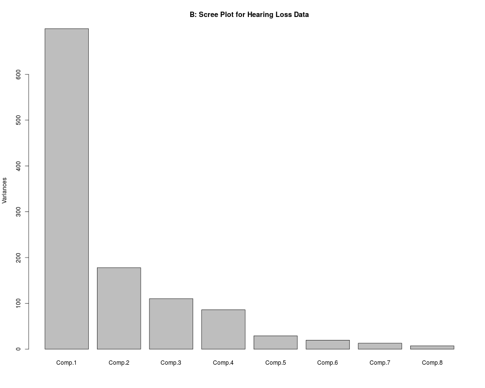
Hearing Loss Data

Description

A study was carried in the Eastman Kodak Company which involved the measurement of hearing loss. Such studies are called as audiometric study. This data set contains 100 males, each aged 39, who had no indication of noise exposure or hearing disorders. Here, the individual is exposed to a signal of a given frequency with an increasing intensity till the signal is perceived.

Usage

data(hearing)

Format

A data frame with 100 observations on the following 9 variables.

Sl_No

Serial Number

L500

Observation for 500Hz in the left ear

L1000

Observation for 1000Hz in the left ear

L2000

Observation for 2000Hz in the left ear

L4000

Observation for 4000Hz in the left ear

R500

Observation for 500Hz in the right ear

R1000

Observation for 1000Hz in the right ear

R2000

Observation for 2000Hz in the right ear

R4000

Observation for 4000Hz in the right ear

References

Jackson, J.E. (1991). A User's Guide to Principal Components. New York: Wiley.

Examples

data(hearing)
round(cor(hearing[,-1]),2)
round(cov(hearing[,-1]),2)
hearing.pc <- princomp(hearing[,-1])
screeplot(hearing.pc,main="B: Scree Plot for Hearing Loss Data")

Results

R version 3.3.1 (2016-06-21) -- "Bug in Your Hair"
Copyright (C) 2016 The R Foundation for Statistical Computing
Platform: x86_64-pc-linux-gnu (64-bit)

R is free software and comes with ABSOLUTELY NO WARRANTY.
You are welcome to redistribute it under certain conditions.
Type 'license()' or 'licence()' for distribution details.

R is a collaborative project with many contributors.
Type 'contributors()' for more information and
'citation()' on how to cite R or R packages in publications.

Type 'demo()' for some demos, 'help()' for on-line help, or
'help.start()' for an HTML browser interface to help.
Type 'q()' to quit R.

> library(ACSWR)
> png(filename="/home/ddbj/snapshot/RGM3/R_CC/result/ACSWR/hearing.Rd_%03d_medium.png", width=480, height=480)
> ### Name: hearing
> ### Title: Hearing Loss Data
> ### Aliases: hearing
> ### Keywords: principal component analysis
> 
> ### ** Examples
> 
> data(hearing)
> round(cor(hearing[,-1]),2)
      L500 L1000 L2000 L4000 R500 R1000 R2000 R4000
L500  1.00  0.78  0.40  0.26 0.70  0.64  0.24  0.20
L1000 0.78  1.00  0.54  0.27 0.55  0.71  0.36  0.22
L2000 0.40  0.54  1.00  0.43 0.24  0.45  0.70  0.33
L4000 0.26  0.27  0.43  1.00 0.18  0.26  0.32  0.71
R500  0.70  0.55  0.24  0.18 1.00  0.66  0.16  0.13
R1000 0.64  0.71  0.45  0.26 0.66  1.00  0.41  0.22
R2000 0.24  0.36  0.70  0.32 0.16  0.41  1.00  0.37
R4000 0.20  0.22  0.33  0.71 0.13  0.22  0.37  1.00
> round(cov(hearing[,-1]),2)
       L500 L1000  L2000  L4000  R500 R1000 R2000  R4000
L500  41.07 37.73  28.13  32.10 31.79 26.30 14.12  25.28
L1000 37.73 57.32  44.44  40.83 29.75 34.24 25.30  31.74
L2000 28.13 44.44 119.70  91.21 18.64 31.21 71.26  68.99
L4000 32.10 40.83  91.21 384.78 25.01 33.03 57.67 269.12
R500  31.79 29.75  18.64  25.01 50.75 30.23 10.52  18.19
R1000 26.30 34.24  31.21  33.03 30.23 40.92 24.62  27.22
R2000 14.12 25.30  71.26  57.67 10.52 24.62 86.30  67.26
R4000 25.28 31.74  68.99 269.12 18.19 27.22 67.26 373.66
> hearing.pc <- princomp(hearing[,-1])
> screeplot(hearing.pc,main="B: Scree Plot for Hearing Loss Data")
> 
> 
> 
> 
> 
> dev.off()
null device 
          1 
>