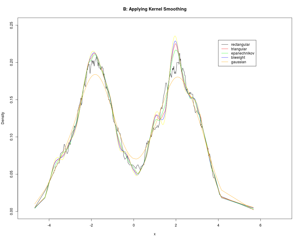
Understanding kernel smoothing through a simulated dataset

Description

This is a simulated dataset with two modes at -2 and 2 and we have 400 observations.

Usage

data(x_bimodal)

Format

The format is: num [1:400] -4.68 -4.19 -4.05 -4.04 -4.02 ...

Examples

data(x_bimodal)
h <- 0.5; n <- length(x_bimodal)
dens_unif <- NULL; dens_triangle <- NULL; dens_epanechnikov <- NULL
dens_biweight <- NULL; dens_triweight <- NULL; dens_gaussian <- NULL
for(i in 1:n)  {
  u <- (x_bimodal[i]-x_bimodal)/h
  xlogical <- (u>-1 & u <= 1)
  dens_unif[i] <- (1/(n*h))*(sum(xlogical)/2)
  dens_triangle[i] <- (1/(n*h))*(sum(xlogical*(1-abs(u))))
  dens_epanechnikov[i] <- (1/(n*h))*(sum(3*xlogical*(1-u^2)/4))
  dens_biweight[i] <- (1/(n*h))*(15*sum(xlogical*(1-u^2)^2/16))
  dens_triweight[i] <- (1/(n*h))*(35*sum(xlogical*(1-u^2)^3/32))
  dens_gaussian[i] <- (1/(n*h))*(sum(exp(-u^2/2)/sqrt(2*pi)))
}
plot(x_bimodal,dens_unif,"l",ylim=c(0,.25),xlim=c(-5,7),xlab="x",
     ylab="Density",main="B: Applying Kernel Smoothing")
points(x_bimodal,dens_triangle,"l",col="red")
points(x_bimodal,dens_epanechnikov,"l",col="green")
points(x_bimodal,dens_biweight,"l",col="blue")
points(x_bimodal,dens_triweight,"l",col="yellow")
points(x_bimodal,dens_gaussian,"l",col="orange")
legend(4,.23,legend=c("rectangular","triangular","epanechnikov","biweight",
                      "gaussian"),col=c("black","red","green","blue","orange"),lty=1)

Results

R version 3.3.1 (2016-06-21) -- "Bug in Your Hair"
Copyright (C) 2016 The R Foundation for Statistical Computing
Platform: x86_64-pc-linux-gnu (64-bit)

R is free software and comes with ABSOLUTELY NO WARRANTY.
You are welcome to redistribute it under certain conditions.
Type 'license()' or 'licence()' for distribution details.

R is a collaborative project with many contributors.
Type 'contributors()' for more information and
'citation()' on how to cite R or R packages in publications.

Type 'demo()' for some demos, 'help()' for on-line help, or
'help.start()' for an HTML browser interface to help.
Type 'q()' to quit R.

> library(ACSWR)
> png(filename="/home/ddbj/snapshot/RGM3/R_CC/result/ACSWR/x_bimodal.Rd_%03d_medium.png", width=480, height=480)
> ### Name: x_bimodal
> ### Title: Understanding kernel smoothing through a simulated dataset
> ### Aliases: x_bimodal
> ### Keywords: kernel smoothing
> 
> ### ** Examples
> 
> data(x_bimodal)
> h <- 0.5; n <- length(x_bimodal)
> dens_unif <- NULL; dens_triangle <- NULL; dens_epanechnikov <- NULL
> dens_biweight <- NULL; dens_triweight <- NULL; dens_gaussian <- NULL
> for(i in 1:n)  {
+   u <- (x_bimodal[i]-x_bimodal)/h
+   xlogical <- (u>-1 & u <= 1)
+   dens_unif[i] <- (1/(n*h))*(sum(xlogical)/2)
+   dens_triangle[i] <- (1/(n*h))*(sum(xlogical*(1-abs(u))))
+   dens_epanechnikov[i] <- (1/(n*h))*(sum(3*xlogical*(1-u^2)/4))
+   dens_biweight[i] <- (1/(n*h))*(15*sum(xlogical*(1-u^2)^2/16))
+   dens_triweight[i] <- (1/(n*h))*(35*sum(xlogical*(1-u^2)^3/32))
+   dens_gaussian[i] <- (1/(n*h))*(sum(exp(-u^2/2)/sqrt(2*pi)))
+ }
> plot(x_bimodal,dens_unif,"l",ylim=c(0,.25),xlim=c(-5,7),xlab="x",
+      ylab="Density",main="B: Applying Kernel Smoothing")
> points(x_bimodal,dens_triangle,"l",col="red")
> points(x_bimodal,dens_epanechnikov,"l",col="green")
> points(x_bimodal,dens_biweight,"l",col="blue")
> points(x_bimodal,dens_triweight,"l",col="yellow")
> points(x_bimodal,dens_gaussian,"l",col="orange")
> legend(4,.23,legend=c("rectangular","triangular","epanechnikov","biweight",
+                       "gaussian"),col=c("black","red","green","blue","orange"),lty=1)
> 
> 
> 
> 
> 
> dev.off()
null device 
          1 
>