R Graphical Manual

Browse All

Last data update: 2014.03.03

R: ADDT Model Fitting

addt.fit

R Documentation

ADDT Model Fitting

Description

Performs the least squares and maximum likelihood procedures for calculating thermal indices (TI) for polymeric materials.

Usage

addt.fit(formula, data, initial.val = 100, proc = "Both",     
    failure.threshold, time.rti = 1e+05, method = "Nelder-Mead",
    subset, na.action, starts = NULL, fail.thres.vec = c(70, 80),            
    ...)

Arguments

`formula`	A formula of type Response~Time+Temperature. The order of Time and Temperature cannot be changed.
`data`	A data frame containing the ADDT data to be analyzed.
`initial.val`	If the data don't contain measurements at time 0, the user needs to specify the initial value for the response. Otherwise, the measurements at time 0 will be used. Default is 100.
`proc`	The type of analysis to be performed. Can be "LS" (least squares), "ML" (maximum likelihood), or "Both" (least squares and maximum likelihood).
`failure.threshold`	The value below which a soft failure occurs. Currently must be in the form of a percent of the initial value. See the example for usage.
`time.rti`	The time associated with the thermal index (TI) or relative thermal index (RTI). Typically 100,000 hours.
`method`	An argument passed to optim specifying the optimization procedure. Default is `"Nelder-Mead"`.
`subset`	An optional statement that allows the use of only part of the dataset.
`na.action`	Indicates the action required when data contain missing values.
`starts`	A vector of starting values for the maximum likelihood procedure. See `fail.thres.vec` for alternative.
`fail.thres.vec`	If the user does not specify "starts" argument, the user may instead specify a vector of two different failure.thresholds. The least square procedure is then used for the two different failure.thresholds to produce starting values for the maximum likelihood procedure.
`...`	Optional arguments.

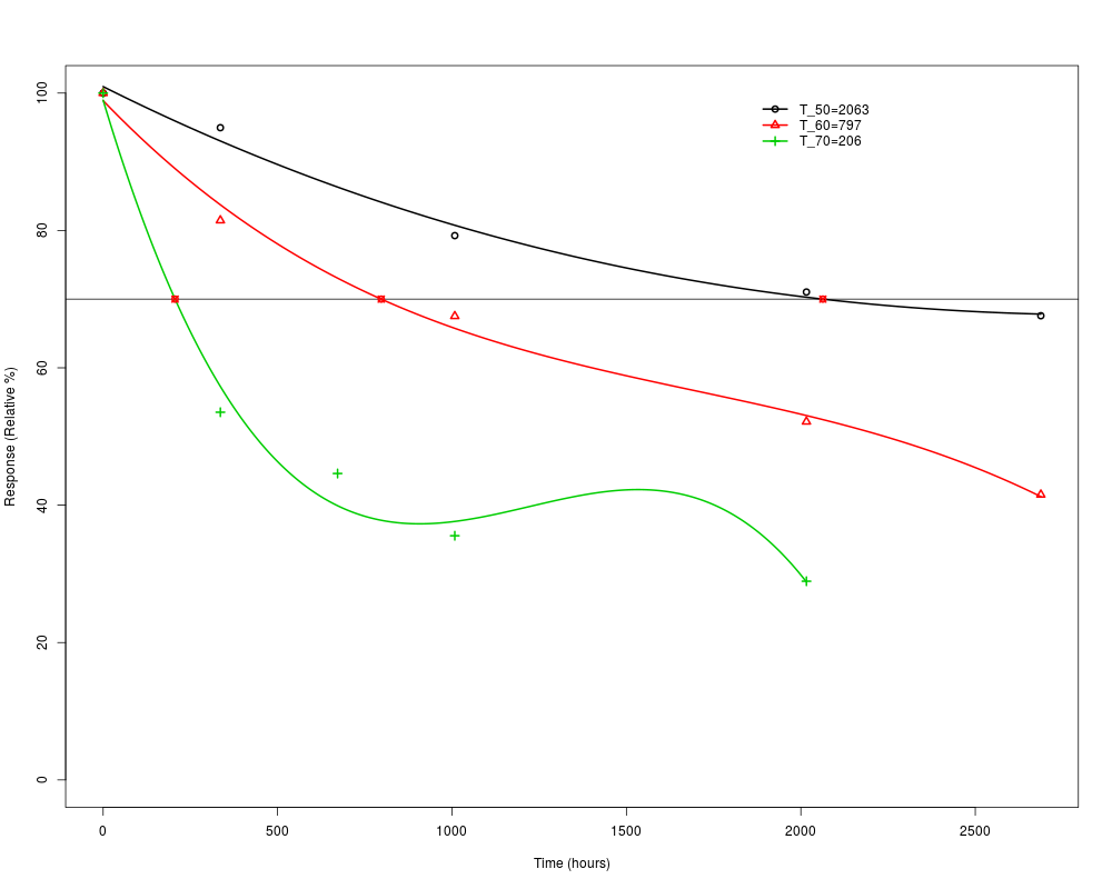
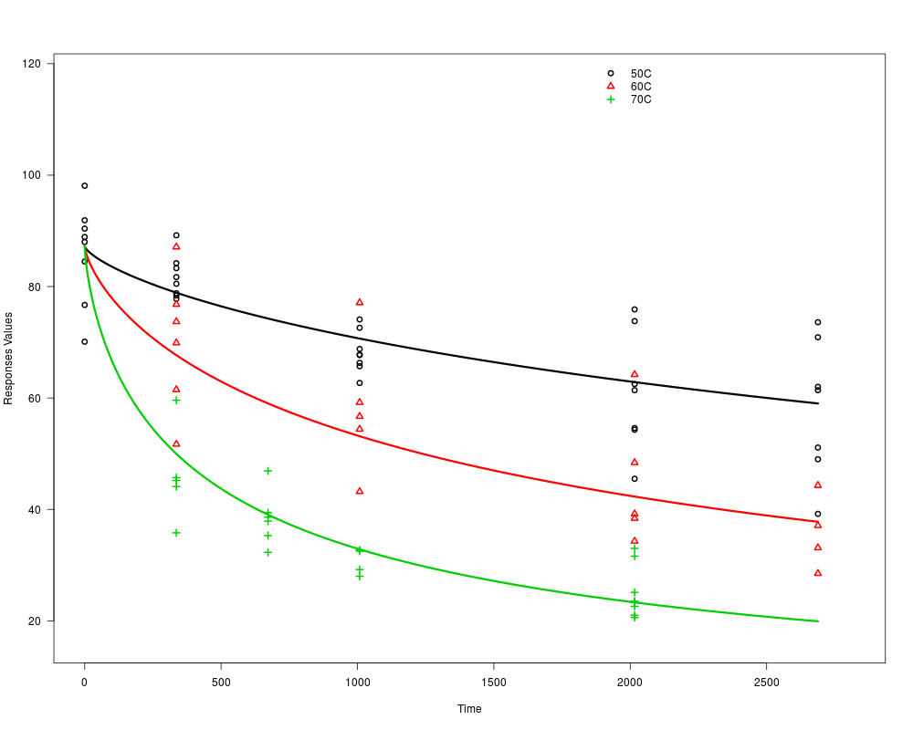
Details

A thermal index (TI) or relative thermal index (RTI) is often used to evaluate long-term performance of polymeric materials. Accelerated destructive degradation testing (ADDT) is widely used to calculate the TI of certain polymeric materials. The least squares and maximum likelihood procedures are the most common procedures used to estimate TI.

The dataset considered in addt.fit function contain repeated measurements of a response, say tensile strength, at some combinations of time and temperature.

The least squares procedure aggregates data into the average of measurements at each combination of time and temperature. Then, polynominal regression is used to interpolate the failure time for each combination. A least squares line is fitted to the failure time data and the TI is then obtained by

TI=frac{beta1}{log10(time.rti)-beta0}-273.16.

It is important to note that observations are required after failure in order for this procedure to be successful.

The maximum likelihood procedure assumes a degradation path dependent on time and temperature. An example of a parametric form for this path can be found in Vaca-Trigo and Meeker (2009) and is the form currently used here. The error term is assumed to follow a multivariate normal distribution. A TI can be directly estimated from the parameter estimates for the degradation path. The addt.fit function will be generalized to allow other parametric forms of the mean function, and/or other non-Guassian distribution in later versions.

Value

An object of class "addt.fit", which is a list containing:

`LS.obj`	If least square approach is used, a LS.obj will returned. It contains estimates of coefficients in the TI formula, estimated TI, a matrix contains the failure time by polynomial interpolation.
`ML.obj`	A ML.obj object is returned if maximum likelihood approach is specified.
`dat`	The data set used in least square/maximum likelihood approaches.
`time.rti`	An argument stored to be used for functions related to "addt.fit" object.
`initial.val`	An argument stored to be used for functions related to "addt.fit" object.
`failure.threshold`	An argument stored to be used for functions related to "addt.fit" object.

References

Hong, Y., King, C. B., Xie, Y., Van Mullekom, J. H., Dehart, S. P. and DeFeo, P. A. (2014). A Comparison of Least Squares and Maximum Likelihood Approaches to Estimating Thermal Indices for Polymeric Materials. Technical Report.

Vaca-Trigo, I. and W. Q. Meeker (2009). A statistical model for linking field and laboratory exposure results for a model coating. NY: New York: Springer.

Examples

data(AdhesiveBondB)

## Least Squares
addt.fit.lsa<-addt.fit(Response~TimeH+TempC,data=AdhesiveBondB,proc="LS",
failure.threshold=70)

## Maximum Likelihood
addt.fit.mla<-addt.fit(Response~TimeH+TempC,data=AdhesiveBondB,proc="ML",
failure.threshold=70)

## Both LS and ML procedures
addt.fit.both<-addt.fit(Response~TimeH+TempC,data=AdhesiveBondB,proc="Both",
failure.threshold=70)

summary(addt.fit.lsa)
summary(addt.fit.mla)
summary(addt.fit.both)

plot(addt.fit.both, type="data")
plot(addt.fit.both, type="LS")
plot(addt.fit.both, type="ML")

addt.confint.ti.mle(addt.fit.mla,conflevel=0.95)

Results


R version 3.3.1 (2016-06-21) -- "Bug in Your Hair"
Copyright (C) 2016 The R Foundation for Statistical Computing
Platform: x86_64-pc-linux-gnu (64-bit)

R is free software and comes with ABSOLUTELY NO WARRANTY.
You are welcome to redistribute it under certain conditions.
Type 'license()' or 'licence()' for distribution details.

R is a collaborative project with many contributors.
Type 'contributors()' for more information and
'citation()' on how to cite R or R packages in publications.

Type 'demo()' for some demos, 'help()' for on-line help, or
'help.start()' for an HTML browser interface to help.
Type 'q()' to quit R.

> library(ADDT)
> png(filename="/home/ddbj/snapshot/RGM3/R_CC/result/ADDT/addt.fit.Rd_%03d_medium.png", width=480, height=480)
> ### Name: addt.fit
> ### Title: ADDT Model Fitting
> ### Aliases: addt.fit
> 
> ### ** Examples
> 
> data(AdhesiveBondB)
> 
> ## Least Squares
> addt.fit.lsa<-addt.fit(Response~TimeH+TempC,data=AdhesiveBondB,proc="LS",
+ failure.threshold=70)
> 
> ## Maximum Likelihood
> addt.fit.mla<-addt.fit(Response~TimeH+TempC,data=AdhesiveBondB,proc="ML",
+ failure.threshold=70)
> 
> ## Both LS and ML procedures
> addt.fit.both<-addt.fit(Response~TimeH+TempC,data=AdhesiveBondB,proc="Both",
+ failure.threshold=70)
> 
> summary(addt.fit.lsa)
Least Squares Approach: 
    beta0     beta1 
 -13.7805 5535.0907 
est.TI: 22 
Interpolation time: 
     Temp      Time
[1,]   50 2063.0924
[2,]   60  797.1901
[3,]   70  206.1681
> summary(addt.fit.mla)

 Maximum Likelihood Approach: 
Call:
lifetime.mle(dat = dat0, minusloglik = minus.loglik.kinetics, 
    starts = starts, method = method, control = list(maxit = 1e+05))

Parameters:
            mean       std  95% Lower  95% Upper
alpha    87.2126    2.5918    82.2778    92.4433
beta0   -37.2489    4.6481   -46.3592   -28.1386
beta1 14917.4450 1562.2183 11855.4972 17979.3928
gamma     0.7272    0.0870     0.5752     0.9194
sigma     8.2007    0.6403     7.0370     9.5569
rho       0.0000    0.0004    -0.0007     0.0007

TI: 
      est       std 95% Lower 95% Upper 
  25.6253    3.0988   19.5518   31.6988 

Loglikelihod:
[1] -288.9057
> summary(addt.fit.both)
Least Squares Approach: 
    beta0     beta1 
 -13.7805 5535.0907 
est.TI: 22 
Interpolation time: 
     Temp      Time
[1,]   50 2063.0924
[2,]   60  797.1901
[3,]   70  206.1681

 Maximum Likelihood Approach: 
Call:
lifetime.mle(dat = dat0, minusloglik = minus.loglik.kinetics, 
    starts = starts, method = method, control = list(maxit = 1e+05))

Parameters:
            mean       std  95% Lower  95% Upper
alpha    87.2126    2.5918    82.2778    92.4433
beta0   -37.2489    4.6481   -46.3592   -28.1386
beta1 14917.4450 1562.2183 11855.4972 17979.3928
gamma     0.7272    0.0870     0.5752     0.9194
sigma     8.2007    0.6403     7.0370     9.5569
rho       0.0000    0.0004    -0.0007     0.0007

TI: 
      est       std 95% Lower 95% Upper 
  25.6253    3.0988   19.5518   31.6988 

Loglikelihod:
[1] -288.9057
> 
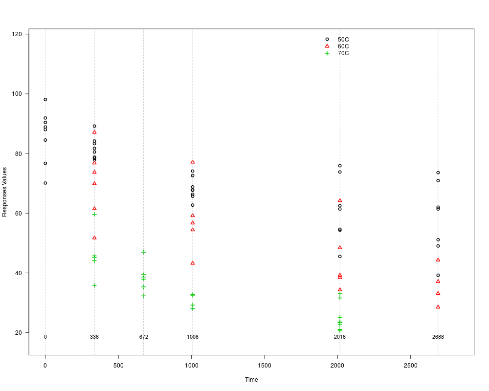
> plot(addt.fit.both, type="data")
> plot(addt.fit.both, type="LS")
     Temp      Time
[1,]   50 2063.0924
[2,]   60  797.1901
[3,]   70  206.1681
> plot(addt.fit.both, type="ML")
> 
> addt.confint.ti.mle(addt.fit.mla,conflevel=0.95)
     est.      s.e.     lower     upper 
25.625268  3.098778 19.551774 31.698762 
> 
> 
> 
> 
> 
> dev.off()
null device 
          1 
>