R Graphical Manual

Browse All

Last data update: 2014.03.03

R: Fast Clustering Using Adaptive Density Peak Detection

adpclust

R Documentation

Fast Clustering Using Adaptive Density Peak Detection

Description

Clustering of data by finding cluster centers from estimated density peaks. It is a non-iterative procedure that incorporates multivariate Gaussian density estimation. The number of clusters as well as bandwidths can either be selected by the user or selected automatically through an internal clustering criterion.

Usage

adpclust(dat, h = NULL, htype = "AMISE", nclust = 2:10,
  centroids = "auto", ac = 1, f.cut = 0.1, fdelta = "mnorm",
  mycols = NULL, dmethod = "euclidean", verbose = FALSE, draw = TRUE,
  findSil = TRUE)

Arguments

`dat`	numeric data frame where rows are observations and columns are variables.
`h`	nonnegative number specifying the bandwidth in density estimation NULL (default). If h is NULL, the algorithm will attempt to find h in a neighborhood centered at either the AMISE bandwidth or ROT bandwidth (see htype).
`htype`	character string specifying the method used to calculate a reference bandwidth for the density estimation. 'htype' is ignored if h is not NULL. Currently the two possible choices of 'htype' are "ROT" and "AMISE" (see details).
`nclust`	integer, or integer vector specifying the pool of the number of clusters in automatic variation. Default is 2:10.
`centroids`	character string specifying "user" or "auto" selection of cluster centroids.
`ac`	integer indicating which automatic cut method is used. Currently it takes one of two values: ac = 1: in the f vs. delta decision plot, 'nclust' points with f > percentile f.cut and nclust largest delta's are declaired centroids. ac = 2: in the f vs. delta decision plot, denote by l the diagonal line connecting the point with smallest f and largest delta, and the point with largest f and smallest delta. 'nclust' points that are above l, and have are farthest away from l are declared centroids.
`f.cut`	number between (0, 1) or numeric vector of numbers between (0,1). f.cut is used in centroids = "auto" to automatically select cluster centroids from the decision plot. Points with f(x) > f.cut and high delta(x) are selected as one set of candidate centroids (see details). Default = c(0.1, 0.2, 0.3).
`fdelta`	character string that specifies the method to estimate densities at each data point. The default (recommended) is "mnorm": multivariate Gaussian density estimation. Other options include normkernel(f <- 1/(h * sqrt(2 * pi)) * rowSums(exp(-(distm/h)^2/2))); Univariate Gaussian smoother weighted(rho <- rowSums(exp(-(distm/h)^2))); Univariate weighted smoother count(rho <- rowSums(distm < h) - 1); Histogram estimator (used in Rodriguez [2014])
`mycols`	a vector of character strings specifying colors used to distinguish different cluster. If the number of clusters is larger than length(mycols) then mycols is recycled. The default is NULL, then 9 colors from brewer.pal-Set1 are used.
`dmethod`	character string describing distance measures used in dist() to calculate proximity matrix of dat. This is passed to the argument "method" in dist(). Default = "euclidean"
`verbose`	if TRUE progress will be displayed.
`draw`	if TRUE results will be plotted on screen. Same as plot.adpclust(ans), where 'ans' is the outcome of 'adpclust()'
`findSil`	if FALSE silhouette score is NOT calculated, and the field that stores silhouette is set to -Inf. The default is TRUE. This argument is IGNORED if length(h) == 0 or length(h) > 1 or length(nclust) > 1, as silhouette scores are needed to select the best clustering in these cases.

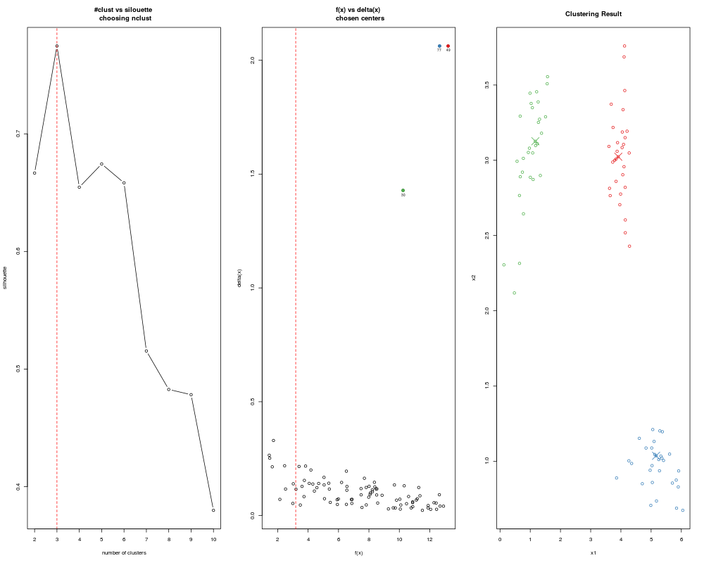
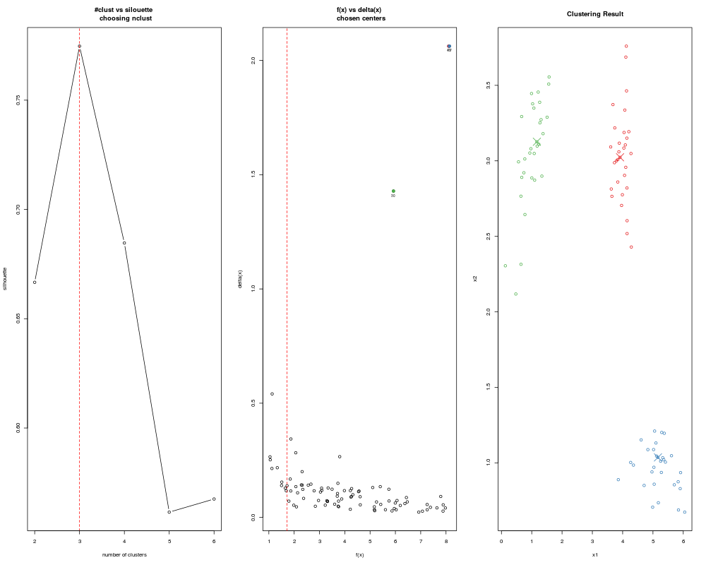
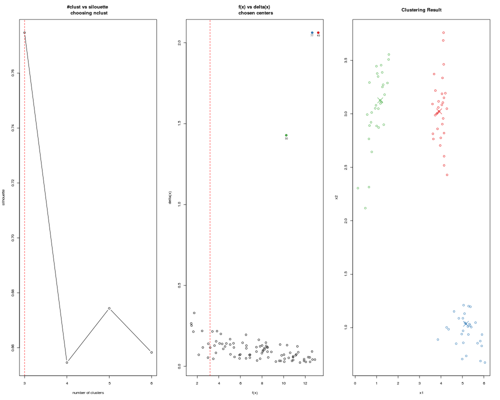
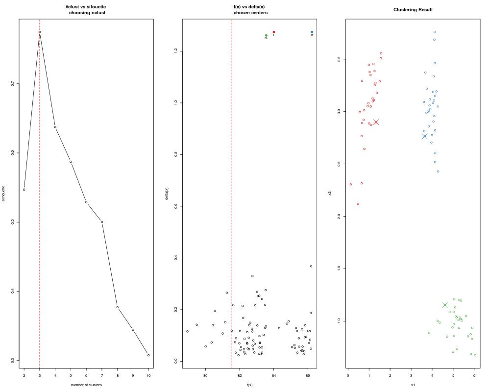
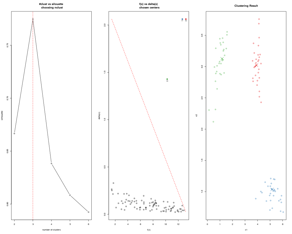
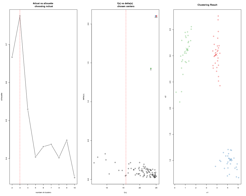
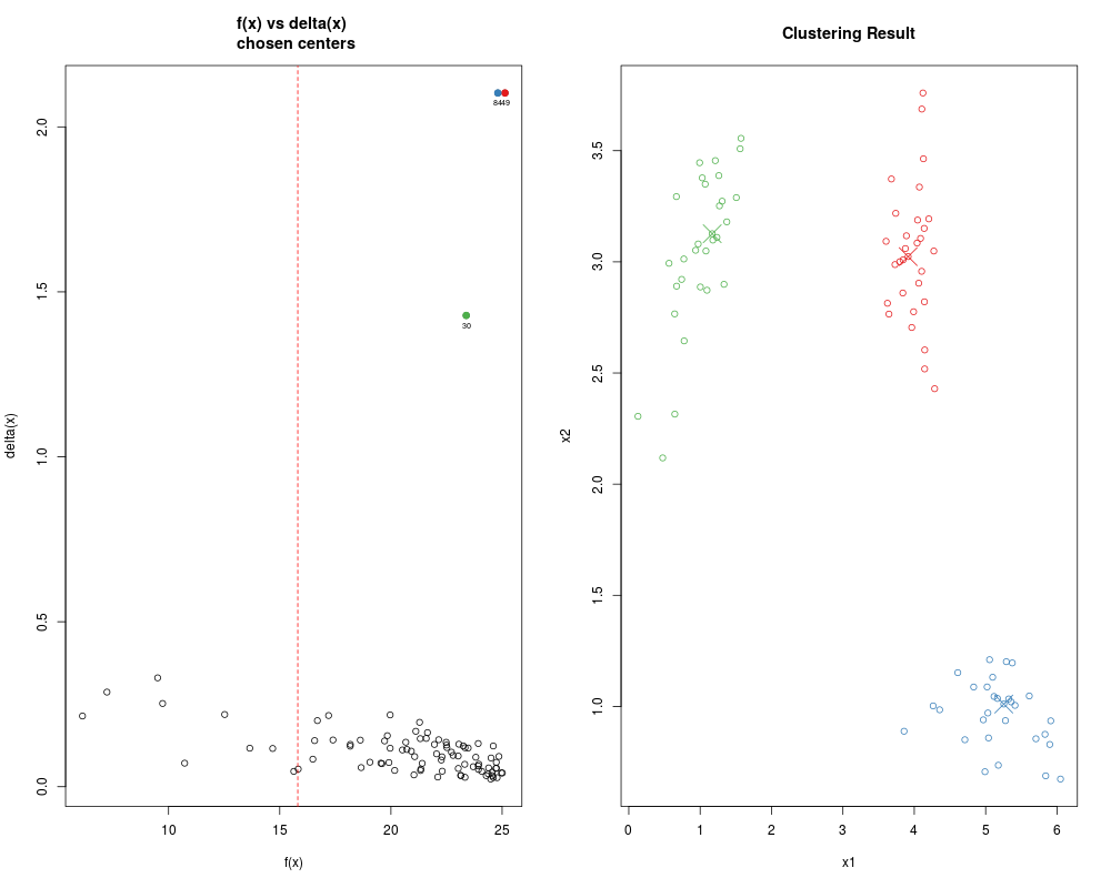
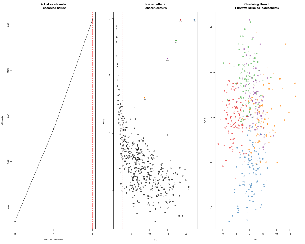
Details

Given n data points in p dimensions, adpclust() first finds local density estimation f(x) of each data point x. The bandwidth h used in density estimation can either be explicitly specified by user through the argument 'h', or automatically selected from a range of testing values. In the case of automatic selection of bandwidths, first a reference bandwidth h0 is calculated by one of the two methods: Scott's Rule-of-Thumb value (htype = "ROT") or Wand's Asymptotic-Mean-Integrated-Squared-Error value (htype = "AMISE"), then 10 values equally spread in the range [1/3h0, 3h0] are tested.

For each data point x, adpclust() also finds an 'isolation' index delta(x), which is defined as the distance between x and the closest point y with f(y) > f(x). The scatter plot (f(x), delta(x)) is called the decision plot. For an appropriate h, cluster centroids appear in the upper-right corner of the decision plot, i.e. points with large f(x) and delta(x). After centroids are picked from the decision plot either by user (centroids = 'user') or automatically (centroids = "auto"), other data points are clustered to the cluster marked by the closest centroid.

When centroids = 'user', the decision plot is generated and displayed on screen. The user selects centroids by clicking the points on the upper right corner of the decision plot. A right click or ESC ends the selection.

Value

An 'adpclust' object, which contains the list of the following items.

f: Final density values (f) for each data point.
delta: Final delta values for each data point.
icenters: Indices of the clustering centers.
clusters Cluster assignments.
score: Silhouette scores.
cut.type: Type of cut used in the automatic variation (see 'ac' argument).
cutvalue: The final best cut value.
h: Best bandwidth.
hs: Bandwidths tried in the automatic selection of bandwidth.

References

GitHub: https://github.com/ethanyxu/ADPclust
Xiao-Feng Wang, and Yifan Xu, (2015) "Fast Clustering Using Adaptive Density Peak Detection." Statistical Methods in Medical Research, doi:10.1177/0962280215609948.
PubMed: http://www.ncbi.nlm.nih.gov/pubmed/26475830

Examples

## Load a data set with 3 clusters
data(clust3)

## Automatically select cluster centroids
ans <- adpclust(clust3, centroids = "auto", draw = FALSE)
summary(ans)
plot(ans)

## Specify the grid of h and nclust
ans <- adpclust(clust3, centroids = "auto", h = c(0.1, 0.2, 0.3), nclust = 2:6)

## Specify that bandwidths should be searched around
## Wand's Asymptotic-Mean-Integrated-Squared-Error bandwidth
## Also test 3 to 6 clusters.
ans <- adpclust(clust3, centroids = "auto", htype = "AMISE", nclust = 3:6)

## Set a specific bandwidth value.
ans <- adpclust(clust3, centroids = "auto", h = 5)

## Change method of automatic selection of centers
ans <- adpclust(clust3, centroids = "auto", nclust = 2:6, ac = 2)

## Specify that the single "ROT" bandwidth value by
## using the 'ROT()' function
ans <- adpclust(clust3, centroids = "auto", h = ROT(clust3))

## Set single h and nclust. Do not calculate silhouette to speed things up
ans <- adpclust(clust3, centroids = "auto", h = ROT(clust3), nclust = 3, findSil = FALSE)

## Centroids selected by user
## Not run: 
ans <- adpclust(clust3, centroids = "user", h = ROT(clust3))

## End(Not run)

## A larger data set
data(clust5)
ans <- adpclust(clust5, centroids = "auto", htype = "ROT", nclust = 3:5)
summary(ans)
plot(ans)

Results


R version 3.3.1 (2016-06-21) -- "Bug in Your Hair"
Copyright (C) 2016 The R Foundation for Statistical Computing
Platform: x86_64-pc-linux-gnu (64-bit)

R is free software and comes with ABSOLUTELY NO WARRANTY.
You are welcome to redistribute it under certain conditions.
Type 'license()' or 'licence()' for distribution details.

R is a collaborative project with many contributors.
Type 'contributors()' for more information and
'citation()' on how to cite R or R packages in publications.

Type 'demo()' for some demos, 'help()' for on-line help, or
'help.start()' for an HTML browser interface to help.
Type 'q()' to quit R.

> library(ADPclust)
> png(filename="/home/ddbj/snapshot/RGM3/R_CC/result/ADPclust/ADPclust.Rd_%03d_medium.png", width=480, height=480)
> ### Name: adpclust
> ### Title: Fast Clustering Using Adaptive Density Peak Detection
> ### Aliases: adpclust
> 
> ### ** Examples
> 
> ## Load a data set with 3 clusters
> data(clust3)
> 
> ## Automatically select cluster centroids
> ans <- adpclust(clust3, centroids = "auto", draw = FALSE)
> summary(ans)
-- ADPclust Procedure -- 

Number of variables: 	 2 
Number of obs.: 	 90 
Centroids selection: 	 Automatic 
Bandwith selection: 	 AMISE (0.16) 
Number of clusters: 	 3 
Avg. Silhouette: 	 0.7747114 

f(x): 
   Min. 1st Qu.  Median    Mean 3rd Qu.    Max. 
  1.444   5.048   7.907   7.599  10.300  13.210 

delta(x): 
   Min. 1st Qu.  Median    Mean 3rd Qu.    Max. 
0.02322 0.05521 0.09144 0.15980 0.13480 2.06300 
> plot(ans)
> 
> ## Specify the grid of h and nclust
> ans <- adpclust(clust3, centroids = "auto", h = c(0.1, 0.2, 0.3), nclust = 2:6)
> 
> ## Specify that bandwidths should be searched around
> ## Wand's Asymptotic-Mean-Integrated-Squared-Error bandwidth
> ## Also test 3 to 6 clusters.
> ans <- adpclust(clust3, centroids = "auto", htype = "AMISE", nclust = 3:6)
> 
> ## Set a specific bandwidth value.
> ans <- adpclust(clust3, centroids = "auto", h = 5)
> 
> ## Change method of automatic selection of centers
> ans <- adpclust(clust3, centroids = "auto", nclust = 2:6, ac = 2)
> 
> ## Specify that the single "ROT" bandwidth value by
> ## using the 'ROT()' function
> ans <- adpclust(clust3, centroids = "auto", h = ROT(clust3))
> 
> ## Set single h and nclust. Do not calculate silhouette to speed things up
> ans <- adpclust(clust3, centroids = "auto", h = ROT(clust3), nclust = 3, findSil = FALSE)
> 
> ## Centroids selected by user
> ## Not run: 
> ##D ans <- adpclust(clust3, centroids = "user", h = ROT(clust3))
> ## End(Not run)
> 
> ## A larger data set
> data(clust5)
> ans <- adpclust(clust5, centroids = "auto", htype = "ROT", nclust = 3:5)
> summary(ans)
-- ADPclust Procedure -- 

Number of variables: 	 5 
Number of obs.: 	 500 
Centroids selection: 	 Automatic 
Bandwith selection: 	 ROT (0.61) 
Number of clusters: 	 5 
Avg. Silhouette: 	 0.2821572 

f(x): 
   Min. 1st Qu.  Median    Mean 3rd Qu.    Max. 
  1.009   4.186   7.208   8.012  11.090  22.240 

delta(x): 
   Min. 1st Qu.  Median    Mean 3rd Qu.    Max. 
 0.2344  0.5645  0.6985  0.7513  0.8686  1.9880 
> plot(ans)
> 
> 
> 
> 
> 
> dev.off()
null device 
          1 
>