R Graphical Manual

Browse All

Last data update: 2014.03.03

R: Attributable fraction function for cohort sampling designs...

AF.ch

R Documentation

Attributable fraction function for cohort sampling designs with time-to-event outcomes.

Description

AF.ch estimates the model-based adjusted attributable fraction function for data from cohort sampling designs with time-to-event outcomes.

Usage

AF.ch(formula, data, exposure, ties = "breslow", times, clusterid)

Arguments

`formula`	a formula object, with the response on the left of a ~ operator, and the terms on the right. The response must be a survival object as returned by the `Surv` function (`Surv`). The exposure and confounders should be specified as independent (right-hand side) variables. The time-to-event outcome should be specified by the survival object. The formula is used to fit a Cox proportional hazards model.
`data`	an optional data frame, list or environment (or object coercible by `as.data.frame` to a data frame) containing the variables in the model. If not found in data, the variables are taken from environment (`formula`), typically the environment from which the function is called.
`exposure`	the name of the exposure variable as a string. The exposure must be binary (0/1) where unexposed is coded as 0.
`ties`	a character string specifying the method for tie handling. If there are no tied death times all the methods are equivalent. Uses the Breslow method by default.
`times`	a scalar or vector of time points specified by the user for which the attributable fraction function is estimated. If not specified the observed death times will be used.
`clusterid`	the name of the cluster identifier variable as a string, if data are clustered.

Details

Af.ch estimates the attributable fraction for a time-to-event outcome under the hypothetical scenario where a binary exposure X is eliminated from the population. The estimate is adjusted for confounders Z by the Cox proportional hazards model (coxph). Let the AF function be defined as

AF = 1 - {1 - S0(t)} / {1 - S(t)}

where S0(t) denotes the counterfactual survival function for the event if the exposure would have been eliminated from the population at baseline and S(t) denotes the factual survival function. If Z is sufficient for confounding control, then S0(t) can be expressed as E_z{S(t|X=0,Z)}. The function uses Cox proportional hazards regression to estimate S(t|X=0,Z), and the marginal sample distribution of Z to approximate the outer expectation (Sj<c3><83><c2><b6>lander and Vansteelandt, 2014). If clusterid is supplied, then a clustered sandwich formula is used in all variance calculations.

Value

`AF.est`	estimated attributable fraction function for every time point specified by `times`.
`AF.var`	estimated variance of `AF.est`. The variance is obtained by combining the delta methods with the sandwich formula.
`S.est`	estimated factual survival function; S(t).
`S.var`	estimated variance of `S.est`. The variance is obtained by the sandwich formula.
`S0.est`	estimated counterfactual survival function if exposure would be eliminated; S0(t).
`S0.var`	estimated variance of `S0.est`. The variance is obtained by the sandwich formula.
`fit`	the fitted model. Fitted using Cox proportional hazard, `coxph`.

Author(s)

Elisabeth Dahlqwist, Arvid Sj<c3><83><c2><b6>lander

References

Chen, L., Lin, D. Y., and Zeng, D. (2010). Attributable fraction functions for censored event times. Biometrika 97, 713-726.

Sj<c3><83><c2><b6>lander, A. and Vansteelandt, S. (2014). Doubly robust estimation of attributable fractions in survival analysis. Statistical Methods in Medical Research. doi: 10.1177/0962280214564003.

Examples

# Simulate a sample from a cohort sampling design with time-to-event outcome
expit <- function(x) 1 / (1 + exp( - x))
n <- 500
time <- c(seq(from = 0.2, to = 1, by = 0.2))
Z <- rnorm(n = n)
X <- rbinom(n = n, size = 1, prob = expit(Z))
Tim <- rexp(n = n, rate = exp(X + Z))
C <- rexp(n = n, rate = exp(X + Z))
Tobs <- pmin(Tim, C)
D <- as.numeric(Tobs < C)
#Ties created by rounding
Tobs <- round(Tobs, digits = 2)

# Example 1: non clustered data from a cohort sampling design with time-to-event outcomes
data <- data.frame(Tobs, D, X,  Z)
AF.est.ch <- AF.ch(formula = Surv(Tobs, D) ~ X + Z + X * Z, data = data,
                   exposure = "X", times = time)
summary(AF.est.ch)

# Example 2: clustered data from a cohort sampling design with time-to-event outcomes
# Duplicate observations in order to create clustered data
id <- rep(1:n, 2)
data <- data.frame(Tobs = c(Tobs, Tobs), D = c(D, D), X = c(X, X), Z = c(Z, Z), id = id)
AF.est.ch.clust <- AF.ch(formula = Surv(Tobs, D) ~ X + Z + X * Z, data = data,
                         exposure = "X", times = time, clusterid = "id")
summary(AF.est.ch.clust)
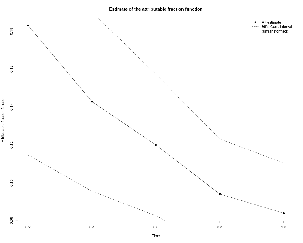
plot(AF.est.ch.clust, CI = TRUE)

Results


R version 3.3.1 (2016-06-21) -- "Bug in Your Hair"
Copyright (C) 2016 The R Foundation for Statistical Computing
Platform: x86_64-pc-linux-gnu (64-bit)

R is free software and comes with ABSOLUTELY NO WARRANTY.
You are welcome to redistribute it under certain conditions.
Type 'license()' or 'licence()' for distribution details.

R is a collaborative project with many contributors.
Type 'contributors()' for more information and
'citation()' on how to cite R or R packages in publications.

Type 'demo()' for some demos, 'help()' for on-line help, or
'help.start()' for an HTML browser interface to help.
Type 'q()' to quit R.

> library(AF)
Loading required package: survival
Loading required package: drgee
Loading required package: nleqslv
Loading required package: Rcpp
Loading required package: data.table
> png(filename="/home/ddbj/snapshot/RGM3/R_CC/result/AF/AF.ch.Rd_%03d_medium.png", width=480, height=480)
> ### Name: AF.ch
> ### Title: Attributable fraction function for cohort sampling designs with
> ###   time-to-event outcomes.
> ### Aliases: AF.ch
> 
> ### ** Examples
> 
> # Simulate a sample from a cohort sampling design with time-to-event outcome
> expit <- function(x) 1 / (1 + exp( - x))
> n <- 500
> time <- c(seq(from = 0.2, to = 1, by = 0.2))
> Z <- rnorm(n = n)
> X <- rbinom(n = n, size = 1, prob = expit(Z))
> Tim <- rexp(n = n, rate = exp(X + Z))
> C <- rexp(n = n, rate = exp(X + Z))
> Tobs <- pmin(Tim, C)
> D <- as.numeric(Tobs < C)
> #Ties created by rounding
> Tobs <- round(Tobs, digits = 2)
> 
> # Example 1: non clustered data from a cohort sampling design with time-to-event outcomes
> data <- data.frame(Tobs, D, X,  Z)
> AF.est.ch <- AF.ch(formula = Surv(Tobs, D) ~ X + Z + X * Z, data = data,
+                    exposure = "X", times = time)
> summary(AF.est.ch)
Call:  
AF.ch(formula = Surv(Tobs, D) ~ X + Z + X * Z, data = data, exposure = "X", 
    times = time)

Estimated attributable fraction (AF) and untransformed 95% Wald CI: 

 Time        AF  Std.Error  z value     Pr(>|z|) Lower limit Upper limit
  0.2 0.3246616 0.06547628 4.958461 7.105367e-07  0.19633045   0.4529927
  0.4 0.2537503 0.04868234 5.212369 1.864444e-07  0.15833467   0.3491659
  0.6 0.2099284 0.03991173 5.259816 1.441993e-07  0.13170281   0.2881539
  0.8 0.1758592 0.03362747 5.229628 1.698511e-07  0.10995053   0.2417678
  1.0 0.1230371 0.02431420 5.060297 4.186045e-07  0.07538212   0.1706920

Exposure : X 
Event    : D 

 Observations Events
          500    243

Method for confounder adjustment:  Cox Proportional Hazards model 

Formula:  Surv(Tobs, D) ~ X + Z + X * Z 
> 
> # Example 2: clustered data from a cohort sampling design with time-to-event outcomes
> # Duplicate observations in order to create clustered data
> id <- rep(1:n, 2)
> data <- data.frame(Tobs = c(Tobs, Tobs), D = c(D, D), X = c(X, X), Z = c(Z, Z), id = id)
> AF.est.ch.clust <- AF.ch(formula = Surv(Tobs, D) ~ X + Z + X * Z, data = data,
+                          exposure = "X", times = time, clusterid = "id")
> summary(AF.est.ch.clust)
Call:  
AF.ch(formula = Surv(Tobs, D) ~ X + Z + X * Z, data = data, exposure = "X", 
    times = time, clusterid = "id")

Estimated attributable fraction (AF) and untransformed 95% Wald CI: 

 Time        AF  Robust SE  z value     Pr(>|z|) Lower limit Upper limit
  0.2 0.3246616 0.04494352 7.223769 5.056617e-13  0.23657392   0.4127493
  0.4 0.2537503 0.03365356 7.540074 4.697059e-14  0.18779054   0.3197101
  0.6 0.2099284 0.02743078 7.653023 1.963095e-14  0.15616502   0.2636917
  0.8 0.1758592 0.02375032 7.404495 1.316504e-13  0.12930938   0.2224089
  1.0 0.1230371 0.01695213 7.257911 3.931140e-13  0.08981151   0.1562627

Exposure : X 
Event    : D 

 Observations Events Clusters
         1000    486      500

Method for confounder adjustment:  Cox Proportional Hazards model 

Formula:  Surv(Tobs, D) ~ X + Z + X * Z 
> plot(AF.est.ch.clust, CI = TRUE)
> 
> 
> 
> 
> 
> dev.off()
null device 
          1 
>