R Graphical Manual

Browse All

Last data update: 2014.03.03

R: Superposes two worm plots

wp.twin

R Documentation

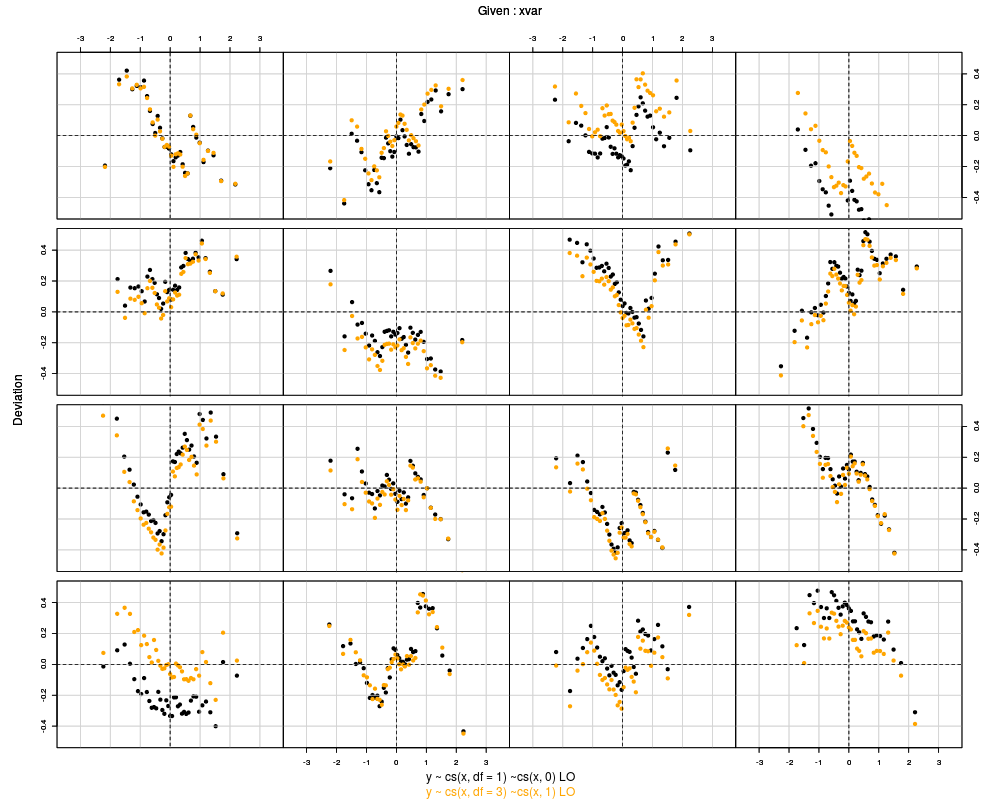
Superposes two worm plots

Description

Superposes two worm plots from GAMLSS fitted objects. This is a diagnostic tool for comparing two solutions.

Usage

wp.twin(obj1, obj2 = NULL, xvar = NULL, xvar.column = 2, n.inter = 16,
  show.given = FALSE, ylim.worm = 0.5, line = FALSE, cex = 1,
  col1 = "black", col2 = "orange", warnings = FALSE, ...)

Arguments

`obj1`	a GAMLSS fitted object
`obj2`	an optional second GAMLSS fitted object
`xvar`	the explanatory variable against which the worm plots will be plotted
`xvar.column`	the number referring to the column of `obj1$mu.x` and `obj2$mu.x`. If `xvar=NULL` then the explanatory variable is set to `xvar=obj1$mu.x[,xvar.column]` respectively `xvar=obj2$mu.x[,xvar.column]`. The default is `xvar.column=2`, which selects the variable following the intercept (which is typically age in most applications).
`n.inter`	the number of intervals in which the explanatory variable `xvar` will be cut. The default is 16.
`show.given`	whether to show the x-variable intervals in the top of the graph, default is `show.given=FALSE`
`ylim.worm`	for multiple plots, this values is the y-variable limit, default value is `ylim.worm=0.5`
`line`	whether to plot the polynomial line in the worm plot, default value is `line=FALSE`
`cex`	the cex plotting parameter with default `cex=1`
`col1`	the color for the points of `obj1`. The default `col="black"`
`col2`	the color for the points of `obj2`. The default `col="orange"`
`warnings`	a logical indicating whether warnings should be produced. The default `warnings=FALSE`
`...`	for extra arguments, `overlap`, `xlim.worm` or `pch`

Details

This function is a customized version of the wp() function found in the gamlss package. Function wp.twin() allows overplotting of two worm plots, each in its own color. The points of obj1 are plotted first, the points of obj2 are superposed. This twin worm plot provide a visual assessment of the differences between the solutions. Extra arguments can be specified (e.g. xvar) that are passed down to the wp() function of gamlss if specified. The worm plot is a detrended normal QQ-plot that highlight departures from normality.

Argument xvar takes priority over xvar.column. The xvar variable is cut into n.iter intervals with an equal number observations and detrended normal QQ (i.e. worm) plots for each interval are plotted. This is a way of highlighting failures of the model within different ranges of the explanatory variable.

If line=TRUE and n.inter>1, the fitted coefficients from fitting cubic polynomials to the residuals (within each x-variable interval) can be obtain by e.g. coeffs<-wp.twin(model1,xvar=x,n.iner=9). van Buuren et al. (2001) used these residuals to identify regions (intervals) of the explanatory variable within which the model does not fit adequately the data (called "model violation")

Value

For multiple plots the xvar intervals and the coefficients of the fitted cubic polynomials to the residuals (within each xvar interval) are returned.

Author(s)

Stef van Buuren, using R code of Mikis Stasinopoulos and Bob Rigby

References

Stasinopoulos D. M. Rigby R.A. (2007) Generalized additive models for location scale and shape (GAMLSS) in R. Journal of Statistical Software, Vol. 23, Issue 7, Dec 2007, http://www.jstatsoft.org/v23/i07.

van Buuren and Fredriks M. (2001) Worm plot: simple diagnostic device for modelling growth reference curves. Statistics in Medicine, 20, 1259–1277.

van Buuren and Fredriks M. (2007) Worm plot to diagnose fit in quantile regression. Statistical Modelling, 7, 4, 363–376.

Examples

library(gamlss)
data(abdom)
a <- gamlss(y~cs(x,df=1),sigma.fo=~cs(x,0),family=LO,data=abdom)
b <- gamlss(y~cs(x,df=3),sigma.fo=~cs(x,1),family=LO,data=abdom)
coeff1 <- wp.twin(a,b,line=TRUE)
coeff1
rm(a,b,coeff1)

Results


R version 3.3.1 (2016-06-21) -- "Bug in Your Hair"
Copyright (C) 2016 The R Foundation for Statistical Computing
Platform: x86_64-pc-linux-gnu (64-bit)

R is free software and comes with ABSOLUTELY NO WARRANTY.
You are welcome to redistribute it under certain conditions.
Type 'license()' or 'licence()' for distribution details.

R is a collaborative project with many contributors.
Type 'contributors()' for more information and
'citation()' on how to cite R or R packages in publications.

Type 'demo()' for some demos, 'help()' for on-line help, or
'help.start()' for an HTML browser interface to help.
Type 'q()' to quit R.

> library(AGD)
AGD 0.35 2015-05-27
> png(filename="/home/ddbj/snapshot/RGM3/R_CC/result/AGD/wp.twin.Rd_%03d_medium.png", width=480, height=480)
> ### Name: wp.twin
> ### Title: Superposes two worm plots
> ### Aliases: wp.twin
> ### Keywords: smooth
> 
> ### ** Examples
> 
> library(gamlss)
Loading required package: splines
Loading required package: gamlss.data
Loading required package: gamlss.dist
Loading required package: MASS
Loading required package: nlme
Loading required package: parallel
 **********   GAMLSS Version 4.4-0  ********** 
For more on GAMLSS look at http://www.gamlss.org/
Type gamlssNews() to see new features/changes/bug fixes.

> data(abdom)
> a <- gamlss(y~cs(x,df=1),sigma.fo=~cs(x,0),family=LO,data=abdom)
GAMLSS-RS iteration 1: Global Deviance = 4795.764 
GAMLSS-RS iteration 2: Global Deviance = 4797.935 
GAMLSS-RS iteration 3: Global Deviance = 4797.948 
GAMLSS-RS iteration 4: Global Deviance = 4797.949 
GAMLSS-RS iteration 5: Global Deviance = 4797.949 
> b <- gamlss(y~cs(x,df=3),sigma.fo=~cs(x,1),family=LO,data=abdom)
GAMLSS-RS iteration 1: Global Deviance = 4781.45 
GAMLSS-RS iteration 2: Global Deviance = 4781.096 
GAMLSS-RS iteration 3: Global Deviance = 4781.118 
GAMLSS-RS iteration 4: Global Deviance = 4781.118 
> coeff1 <- wp.twin(a,b,line=TRUE)
> coeff1
$classes
     [,1]  [,2]
1   12.22 14.64
39  14.64 16.78
77  16.78 18.36
115 18.36 20.07
154 20.07 21.93
192 21.93 23.50
230 23.50 25.07
268 25.07 27.07
306 27.07 28.93
344 28.93 30.64
382 30.64 32.50
420 32.50 34.50
458 34.50 36.21
497 36.21 38.36
535 38.36 40.93
573 40.93 42.50

$coef
              [,1]        [,2]         [,3]         [,4]
 [1,] -0.003504020 -0.15602304  0.038639888  0.027393705
 [2,]  0.026515864  0.28483180  0.006095326 -0.093187380
 [3,] -0.077876298  0.05628599  0.061894229  0.009416131
 [4,]  0.209698618 -0.02456995 -0.034685801 -0.031058629
 [5,] -0.060524040  0.39289973  0.065269080 -0.123323496
 [6,] -0.020070631  0.04750037 -0.043512545 -0.042320484
 [7,] -0.321110690 -0.10433001  0.168580670  0.056075986
 [8,]  0.064037966 -0.05531105 -0.020258555 -0.090437121
 [9,]  0.128936714  0.17913097  0.044109902 -0.049297039
[10,] -0.266363310 -0.01890913  0.017866160 -0.019747330
[11,]  0.007205697 -0.11774411  0.137228619  0.021868979
[12,]  0.201188563  0.15077864 -0.052544238 -0.002615670
[13,]  0.007664226 -0.23640794 -0.009871868  0.039585716
[14,] -0.017449540  0.16811355  0.026607674 -0.009545766
[15,]  0.124703184  0.11954586  0.020848864 -0.035485678
[16,] -0.174190902 -0.16016432 -0.081501991  0.003570043

> rm(a,b,coeff1)
> 
> 
> 
> 
> 
> dev.off()
null device 
          1 
>