Supported by Dr. Osamu Ogasawara and  . . |
|
Last data update: 2014.03.03 |
alternating least squares multivariate curve resolution (MCR-ALS)DescriptionThis is an implementation of alternating least squares
multivariate curve resolution (MCR-ALS). Given a dataset in matrix
form Usage
als(CList, PsiList, S=matrix(), WList=list(),
thresh =.001, maxiter=100, forcemaxiter = FALSE,
optS1st=TRUE, x=1:nrow(CList[[1]]), x2=1:nrow(S),
baseline=FALSE, fixed=vector("list", length(PsiList)),
uniC=FALSE, uniS=FALSE, nonnegC = TRUE, nonnegS = TRUE,
normS=0, closureC=list())
Arguments
ValueA list with components:
NoteThis function was used to solve problems described in van Stokkum IHM, Mullen KM, Mihaleva VV. Global analysis of multiple gas chromatography-mass spectrometry (GS/MS) data sets: A method for resolution of co-eluting components with comparison to MCR-ALS. Chemometrics and Intelligent Laboratory Systems 2009; 95(2): 150-163. in conjunction with the package TIMP. For the code to reproduce
the examples in this paper, see examples_chemo.zip included in the
ReferencesGarrido M, Rius FX, Larrechi MS. Multivariate curve resolution alternating least squares (MCR-ALS) applied to spectroscopic data from monitoring chemical reactions processes. Journal Analytical and Bioanalytical Chemistry 2008; 390:2059-2066. Jonsson P, Johansson A, Gullberg J, Trygg J, A J, Grung B, Marklund S, Sjostrom M, Antti H, Moritz T. High-throughput data analysis for detecting and identifying differences between samples in GC/MS-based metabolomic analyses. Analytical Chemistry 2005; 77:5635-5642. Tauler R. Multivariate curve resolution applied to second order data. Chemometrics and Intelligent Laboratory Systems 1995; 30:133-146. Tauler R, Smilde A, Kowalski B. Selectivity, local rank, three-way data analysis and ambiguity in multivariate curve resolution. Journal of Chemometrics 1995; 9:31-58. See Also
Examples## load 2 matrix datasets into variables d1 and d2 ## load starting values for elution profiles ## into variables Cstart1 and Cstart2 ## load time labels as x, m/z values as x2 data(multiex) ## starting values for elution profiles matplot(x,Cstart1,type="l") matplot(x,Cstart2,type="l",add=TRUE) ## using MCR-ALS, improve estimates for mass spectra S and the two ## matrices of elution profiles ## apply unimodality constraints to the elution profile estimates ## note that the starting estimates for S just contain a dummy matrix test0 <- als(CList=list(Cstart1,Cstart2),S=matrix(1,nrow=400,ncol=2), PsiList=list(d1,d2), x=x, x2=x2, uniC=TRUE, normS=0) ## plot the estimated mass spectra plotS(test0$S,x2) ## the known mass spectra are contained in the variable S ## can compare the matching factor of each estimated spectrum to ## that in S matchFactor(S[,1],test0$S[,1]) matchFactor(S[,2],test0$S[,2]) ## plot the estimated elution profiles ## this shows the relative abundance of the 2nd component is low matplot(x,test0$CList[[1]],type="l") matplot(x,test0$CList[[2]],type="l",add=TRUE) Results
R version 3.3.1 (2016-06-21) -- "Bug in Your Hair"
Copyright (C) 2016 The R Foundation for Statistical Computing
Platform: x86_64-pc-linux-gnu (64-bit)
R is free software and comes with ABSOLUTELY NO WARRANTY.
You are welcome to redistribute it under certain conditions.
Type 'license()' or 'licence()' for distribution details.
R is a collaborative project with many contributors.
Type 'contributors()' for more information and
'citation()' on how to cite R or R packages in publications.
Type 'demo()' for some demos, 'help()' for on-line help, or
'help.start()' for an HTML browser interface to help.
Type 'q()' to quit R.
> library(ALS)
Loading required package: nnls
Loading required package: Iso
Iso 0.0-17
> png(filename="/home/ddbj/snapshot/RGM3/R_CC/result/ALS/als.Rd_%03d_medium.png", width=480, height=480)
> ### Name: als
> ### Title: alternating least squares multivariate curve resolution
> ### (MCR-ALS)
> ### Aliases: als
> ### Keywords: optimize
>
> ### ** Examples
>
> ## load 2 matrix datasets into variables d1 and d2
> ## load starting values for elution profiles
> ## into variables Cstart1 and Cstart2
> ## load time labels as x, m/z values as x2
> data(multiex)
>
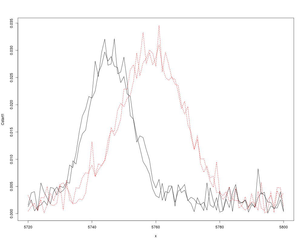
> ## starting values for elution profiles
> matplot(x,Cstart1,type="l")
> matplot(x,Cstart2,type="l",add=TRUE)
>
> ## using MCR-ALS, improve estimates for mass spectra S and the two
> ## matrices of elution profiles
> ## apply unimodality constraints to the elution profile estimates
> ## note that the starting estimates for S just contain a dummy matrix
>
> test0 <- als(CList=list(Cstart1,Cstart2),S=matrix(1,nrow=400,ncol=2),
+ PsiList=list(d1,d2), x=x, x2=x2, uniC=TRUE, normS=0)
Initial RSS 3.039967e+13
Iteration (opt. S): 1, RSS: 1.330703e+12, RD: 0.9562264
Iteration (opt. C): 2, RSS: 153488187, RD: 0.9998847
Iteration (opt. S): 3, RSS: 102433454, RD: 0.3326297
Iteration (opt. C): 4, RSS: 102351694, RD: 0.0007981757
Initial RSS / Final RSS = 3.039967e+13 / 102351694 = 297011.9
>
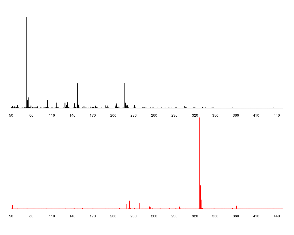
> ## plot the estimated mass spectra
> plotS(test0$S,x2)
>
> ## the known mass spectra are contained in the variable S
> ## can compare the matching factor of each estimated spectrum to
> ## that in S
> matchFactor(S[,1],test0$S[,1])
[,1]
[1,] 0.9999994
> matchFactor(S[,2],test0$S[,2])
[,1]
[1,] 0.9999917
>
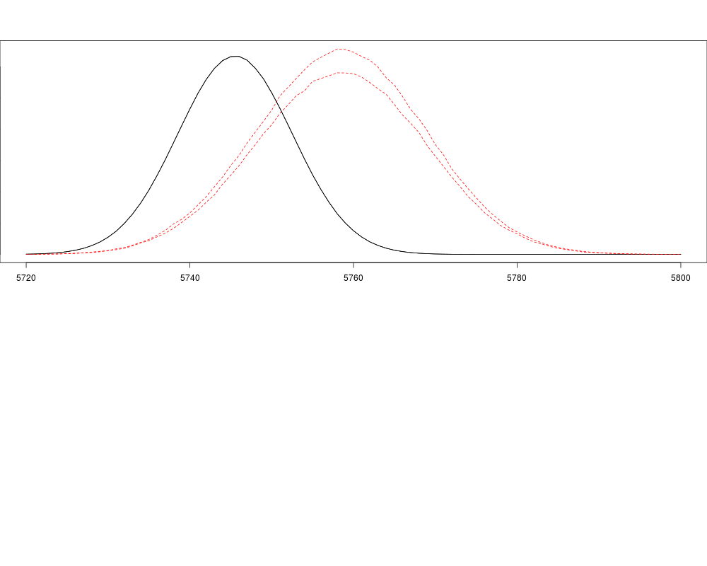
> ## plot the estimated elution profiles
> ## this shows the relative abundance of the 2nd component is low
> matplot(x,test0$CList[[1]],type="l")
> matplot(x,test0$CList[[2]],type="l",add=TRUE)
>
>
>
>
>
> dev.off()
null device
1
>
|