R Graphical Manual

Browse All

Last data update: 2014.03.03

R: Create a Multilayer Feedforward Neural Network

newff

R Documentation

Create a Multilayer Feedforward Neural Network

Description

Creates a feedforward artificial neural network according to the structure established by the AMORE package standard.

Usage

newff(n.neurons, learning.rate.global, momentum.global, error.criterium, Stao, 
	hidden.layer, output.layer, method)

Arguments

`n.neurons`	Numeric vector containing the number of neurons of each layer. The first element of the vector is the number of input neurons, the last is the number of output neurons and the rest are the number of neuron of the different hidden layers.
`learning.rate.global`	Learning rate at which every neuron is trained.
`momentum.global`	Momentum for every neuron. Needed by several training methods.
`error.criterium`	Criterium used to measure to proximity of the neural network prediction to its target. Currently we can choose amongst: "LMS": Least Mean Squares. "LMLS": Least Mean Logarithm Squared (Liano 1996). "TAO": TAO Error (Pernia, 2004).
`Stao`	Stao parameter for the TAO error criterium. Unused by the rest of criteria.
`hidden.layer`	Activation function of the hidden layer neurons. Available functions are: "purelin". "tansig". "sigmoid". "hardlim". "custom": The user must manually define the f0 and f1 elements of the neurons.
`output.layer`	Activation function of the hidden layer neurons according to the former list shown above.
`method`	Prefered training method. Currently it can be: "ADAPTgd": Adaptative gradient descend. "ADAPTgdwm": Adaptative gradient descend with momentum. "BATCHgd": BATCH gradient descend. "BATCHgdwm": BATCH gradient descend with momentum.

Value

newff returns a multilayer feedforward neural network object.

Author(s)

Manuel Castej<c3><83><c2><b3>n Limas. manuel.castejon@gmail.com
Joaquin Ordieres Mer<c3><83><c2><a9>. Ana Gonz<c3><83><c2><a1>lez Marcos. Alpha V. Pern<c3><83><c2><ad>a Espinoza. Eliseo P. Vergara Gonzalez. Francisco Javier Martinez de Pis<c3><83><c2><b3>n. Fernando Alba El<c3><83><c2><ad>as.

References

Pern<c3><83><c2><ad>a Espinoza, A.V., Ordieres Mer<c3><83><c2><a9>, J.B., Mart<c3><83><c2><ad>nez de Pis<c3><83><c2><b3>n, F.J., Gonz<c3><83><c2><a1>lez Marcos, A. TAO-robust backpropagation learning algorithm. Neural Networks. Vol. 18, Issue 2, pp. 191–204, 2005.

Simon Haykin. Neural Networks – a Comprehensive Foundation. Prentice Hall, New Jersey, 2nd edition, 1999. ISBN 0-13-273350-1.

Examples

#Example 1

library(AMORE)
# P is the input vector
P <- matrix(sample(seq(-1,1,length=1000), 1000, replace=FALSE), ncol=1) 
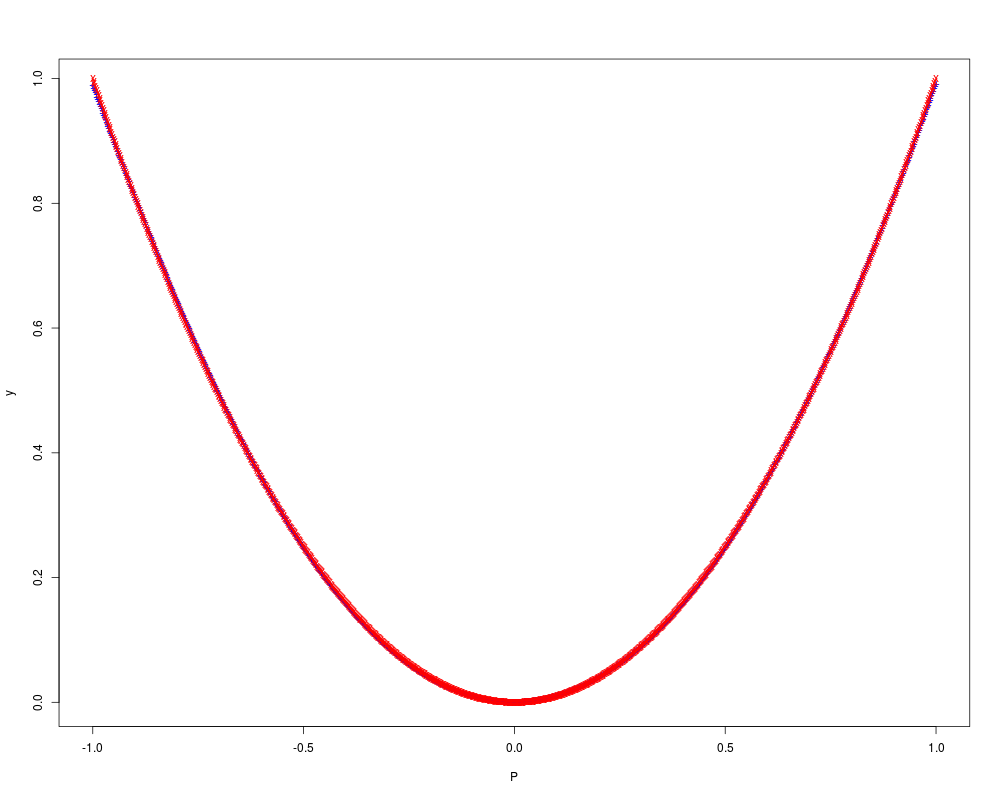
# The network will try to approximate the target P^2
target <- P^2                                   
# We create a feedforward network, with two hidden layers.
# The first hidden layer has three neurons and the second has two neurons.
# The hidden layers have got Tansig activation functions and the output layer is Purelin.
net <- newff(n.neurons=c(1,3,2,1), learning.rate.global=1e-2, momentum.global=0.5,
        error.criterium="LMS", Stao=NA, hidden.layer="tansig", 
        output.layer="purelin", method="ADAPTgdwm")
result <- train(net, P, target, error.criterium="LMS", report=TRUE, show.step=100, n.shows=5 )
y <- sim(result$net, P)
plot(P,y, col="blue", pch="+")
points(P,target, col="red", pch="x")

Results


R version 3.3.1 (2016-06-21) -- "Bug in Your Hair"
Copyright (C) 2016 The R Foundation for Statistical Computing
Platform: x86_64-pc-linux-gnu (64-bit)

R is free software and comes with ABSOLUTELY NO WARRANTY.
You are welcome to redistribute it under certain conditions.
Type 'license()' or 'licence()' for distribution details.

R is a collaborative project with many contributors.
Type 'contributors()' for more information and
'citation()' on how to cite R or R packages in publications.

Type 'demo()' for some demos, 'help()' for on-line help, or
'help.start()' for an HTML browser interface to help.
Type 'q()' to quit R.

> library(AMORE)
> png(filename="/home/ddbj/snapshot/RGM3/R_CC/result/AMORE/newff.Rd_%03d_medium.png", width=480, height=480)
> ### Name: newff
> ### Title: Create a Multilayer Feedforward Neural Network
> ### Aliases: newff
> ### Keywords: neural
> 
> ### ** Examples
> 
> #Example 1
> 
> library(AMORE)
> # P is the input vector
> P <- matrix(sample(seq(-1,1,length=1000), 1000, replace=FALSE), ncol=1) 
> # The network will try to approximate the target P^2
> target <- P^2                                   
> # We create a feedforward network, with two hidden layers.
> # The first hidden layer has three neurons and the second has two neurons.
> # The hidden layers have got Tansig activation functions and the output layer is Purelin.
> net <- newff(n.neurons=c(1,3,2,1), learning.rate.global=1e-2, momentum.global=0.5,
+         error.criterium="LMS", Stao=NA, hidden.layer="tansig", 
+         output.layer="purelin", method="ADAPTgdwm")
> result <- train(net, P, target, error.criterium="LMS", report=TRUE, show.step=100, n.shows=5 )
index.show: 1 LMS 0.0007070751786775 
index.show: 2 LMS 0.000215891795660443 
index.show: 3 LMS 5.31091712266644e-05 
index.show: 4 LMS 8.19184378877529e-06 
index.show: 5 LMS 3.13605377993589e-06 
> y <- sim(result$net, P)
> plot(P,y, col="blue", pch="+")
> points(P,target, col="red", pch="x")
> 
> 
> 
> 
> 
> dev.off()
null device 
          1 
>