R Graphical Manual

Browse All

Last data update: 2014.03.03

R: Operating Characteristics of an Acceptance Sampling Plan

OC2c	R Documentation

Operating Characteristics of an Acceptance Sampling Plan

Description

The preferred way of creating new objects from the family of "OC2c" classes.

Usage

OC2c(n,c,r=if (length(c)==1) c+1 else NULL,
  type=c("binomial","hypergeom", "poisson"), ...)

Arguments

`n`	A vector of length k giving the sample size at each of the k stages of sampling, e.g. for double sampling k=2.
`c`	A vector of length k giving the cumulative acceptance numbers at each of the k stages of sampling.
`r`	A vector of length k giving the cumulative rejection numbers at each of the k stages of sampling.
`type`	The possible types relate to the distribution on which the plans are based on, namely, `binomial`, `hypergeom`, and `poisson`.
`...`	Additional parameters passed to the class generating function for each type. See Details for options.

Details

Typical usages are:

    OC2c(n, c)
    OC2c(n, c, r, pd)
    OC2c(n, c, r, type="hypergeom", N, pd)
    OC2c(n, c, r, type="poisson", pd)

The first and second forms use a default type of "binomial". The first form can calculate r only when n and c are of length 1.

The second form provides a the proportion of defectives, pd, for which the OC function should be calculated (default is pd=seq(0, 1, 0.01).

The third form states that the OC function based on a Hypergeometric distribution is desired. In this case the population size N also needs to be specified. In this case, pd indicates the proportion of population defectives, such that pd*N gives the actual number of defectives in the population. If N or pd are not specified they take defaults of N=100 and pd=seq(0, 1, 0.01).

Value

An object from the family of OC2c-class, namely of class OCbinomial, OChypergeom, or OCpoisson.

Examples

## A standard binomial sampling plan
x <- OC2c(10,1)
x ## print out a brief summary
plot(x) ## plot the OC curve
plot(x, xlim=c(0,0.5)) ## plot the useful part of the OC curve

## A double sampling plan
x <- OC2c(c(125,125), c(1,4), c(4,5), pd=seq(0,0.1,0.001))
x
plot(x) ## Plot the plan

## Assess whether the plan can meet desired risk points
assess(x, PRP=c(0.01, 0.95), CRP=c(0.05, 0.04))

## A plan based on the Hypergeometric distribution
x <- OC2c(10,1, type="hypergeom", N=5000, pd=seq(0,0.5, 0.025))
plot(x)

## The summary
x <- OC2c(10,1, type="hypergeom", N=5000, pd=seq(0,0.5, 0.1))
summary(x, full=TRUE)

## Plotting against a function which generates P(defective)
xm <- seq(-3, 3, 0.05) ## The mean of the underlying characteristic
x <- OC2c(10, 1, pd=1-pnorm(0, mean=xm, sd=1))
plot(xm, x) ## Plot P(accept) against mean

Results


R version 3.3.1 (2016-06-21) -- "Bug in Your Hair"
Copyright (C) 2016 The R Foundation for Statistical Computing
Platform: x86_64-pc-linux-gnu (64-bit)

R is free software and comes with ABSOLUTELY NO WARRANTY.
You are welcome to redistribute it under certain conditions.
Type 'license()' or 'licence()' for distribution details.

R is a collaborative project with many contributors.
Type 'contributors()' for more information and
'citation()' on how to cite R or R packages in publications.

Type 'demo()' for some demos, 'help()' for on-line help, or
'help.start()' for an HTML browser interface to help.
Type 'q()' to quit R.

> library(AcceptanceSampling)
> png(filename="/home/ddbj/snapshot/RGM3/R_CC/result/AcceptanceSampling/OC2c.Rd_%03d_medium.png", width=480, height=480)
> ### Name: OC2c
> ### Title: Operating Characteristics of an Acceptance Sampling Plan
> ### Aliases: OC2c plot,OC2c-method plot,OCbinomial,missing-method
> ###   plot,numeric,OCbinomial-method plot,OChypergeom,missing-method
> ###   plot,numeric,OChypergeom-method plot,OCpoisson,missing-method
> ###   plot,numeric,OCpoisson-method show,OC2c-method
> ###   show,OChypergeom-method summary,OC2c-method
> ###   summary,OChypergeom-method
> ### Keywords: classes
> 
> ### ** Examples
> 
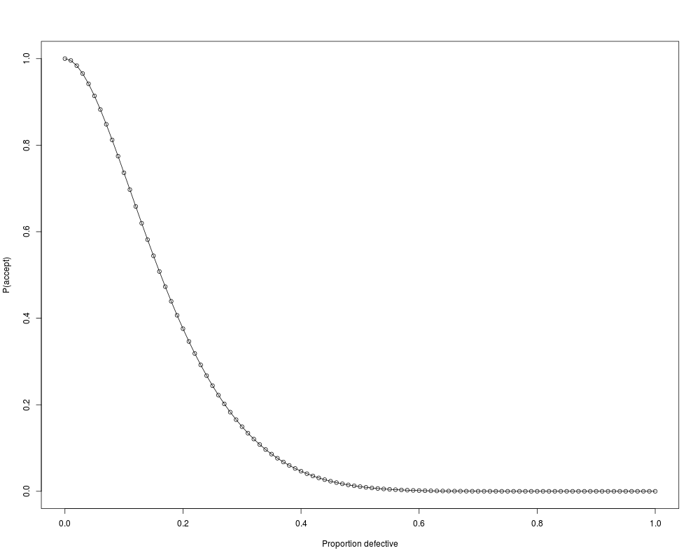
> ## A standard binomial sampling plan
> x <- OC2c(10,1)
> x ## print out a brief summary
Acceptance Sampling Plan (binomial)

               Sample 1
Sample size(s)       10
Acc. Number(s)        1
Rej. Number(s)        2
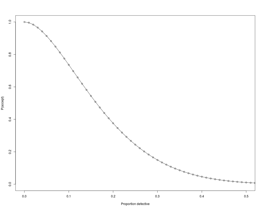
> plot(x) ## plot the OC curve
> plot(x, xlim=c(0,0.5)) ## plot the useful part of the OC curve
> 
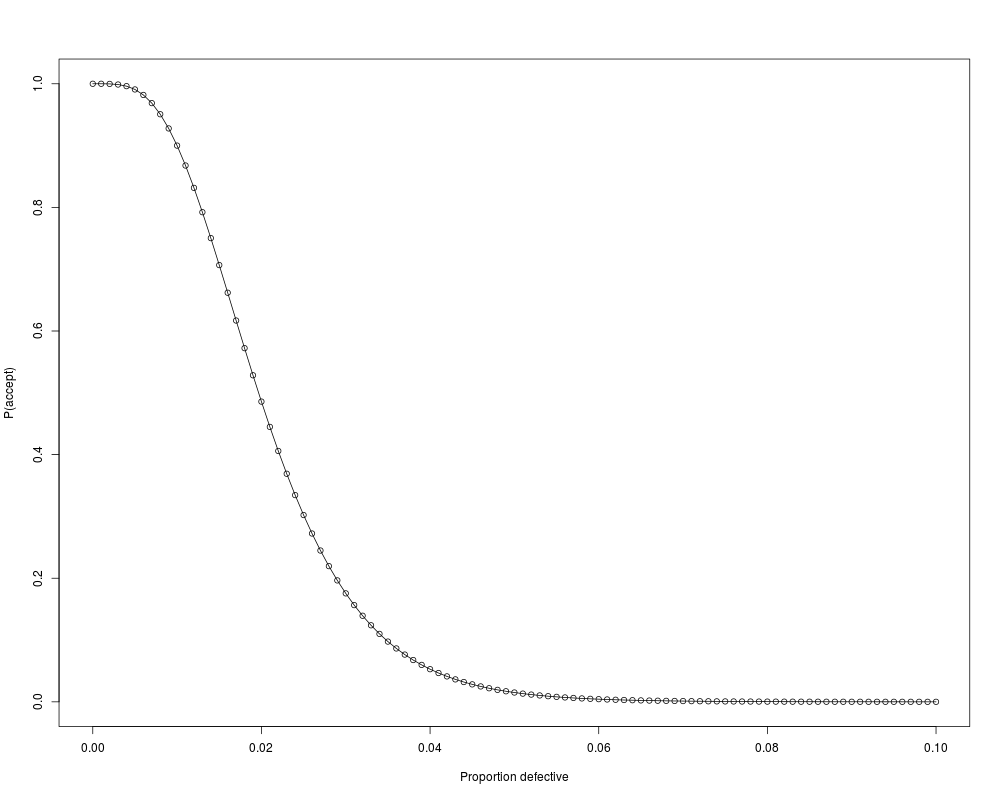
> ## A double sampling plan
> x <- OC2c(c(125,125), c(1,4), c(4,5), pd=seq(0,0.1,0.001))
> x
Acceptance Sampling Plan (binomial)

               Sample 1 Sample 2
Sample size(s)      125      125
Acc. Number(s)        1        4
Rej. Number(s)        4        5
> plot(x) ## Plot the plan
> 
> ## Assess whether the plan can meet desired risk points
> assess(x, PRP=c(0.01, 0.95), CRP=c(0.05, 0.04))
Acceptance Sampling Plan (binomial)

               Sample 1 Sample 2
Sample size(s)      125      125
Acc. Number(s)        1        4
Rej. Number(s)        4        5

Plan CANNOT meet desired risk point(s):

           Quality   RP P(accept) Plan P(accept)
PRP           0.01           0.95     0.89995598
CRP           0.05           0.04     0.01507571
> 
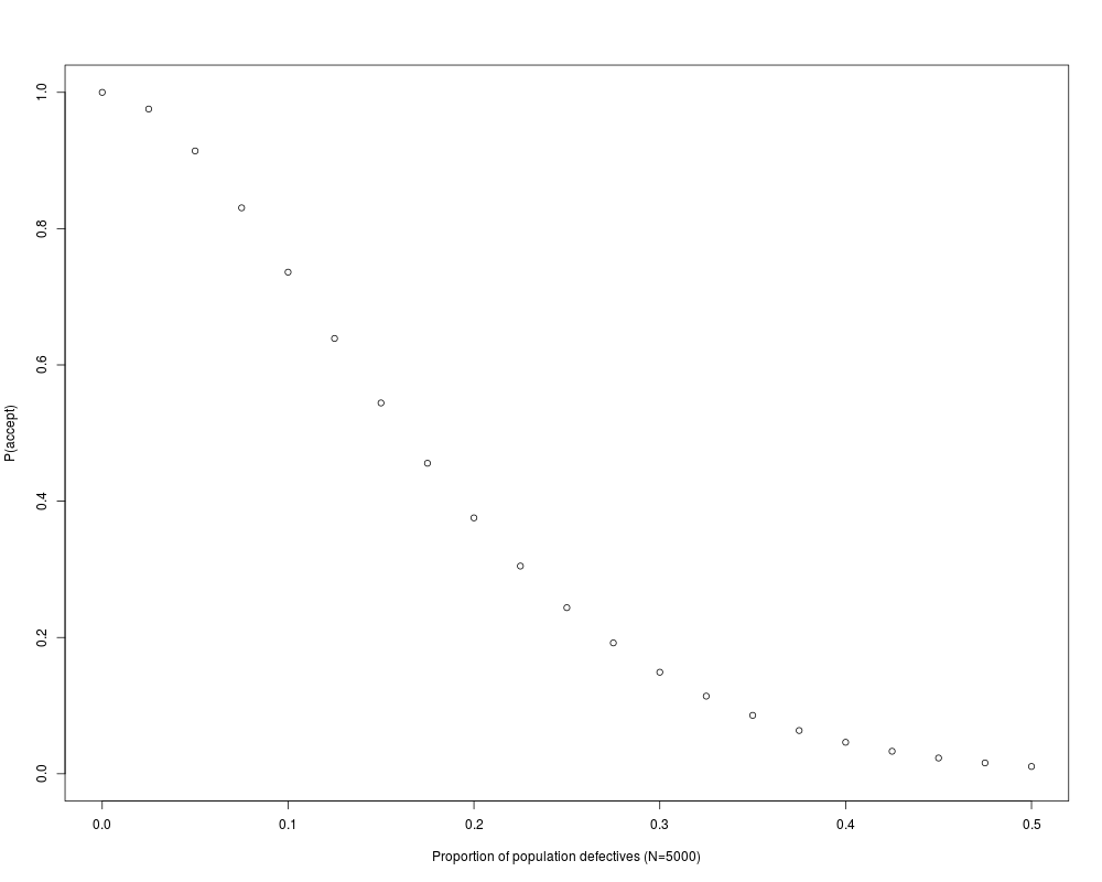
> ## A plan based on the Hypergeometric distribution
> x <- OC2c(10,1, type="hypergeom", N=5000, pd=seq(0,0.5, 0.025))
> plot(x)
> 
> ## The summary
> x <- OC2c(10,1, type="hypergeom", N=5000, pd=seq(0,0.5, 0.1))
> summary(x, full=TRUE)
Acceptance Sampling Plan (hypergeom with N=5000)

               Sample 1
Sample size(s)       10
Acc. Number(s)        1
Rej. Number(s)        2

Detailed acceptance probabilities:

 Pop. Defectives Pop. Prop. defective  P(accept)
               0                  0.0 1.00000000
             500                  0.1 0.73613783
            1000                  0.2 0.37556779
            1500                  0.3 0.14904357
            2000                  0.4 0.04620019
            2500                  0.5 0.01068073
> 
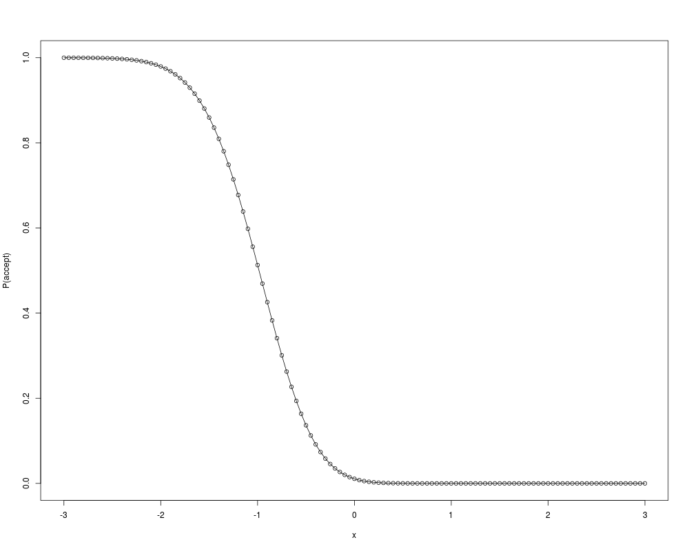
> ## Plotting against a function which generates P(defective)
> xm <- seq(-3, 3, 0.05) ## The mean of the underlying characteristic
> x <- OC2c(10, 1, pd=1-pnorm(0, mean=xm, sd=1))
> plot(xm, x) ## Plot P(accept) against mean
> 
> 
> 
> 
> 
> dev.off()
null device 
          1 
>