Supported by Dr. Osamu Ogasawara and  . . |
|
Last data update: 2014.03.03 |
Fit a semiparametric regression model with spatially adaptive penalized splinesDescription
Usage
asp(form,adap=TRUE,random=NULL,group=NULL,family="gaussian",
                spar.method="REML",omit.missing=NULL,niter=20,niter.var=50,tol=1e-06,returnFit=FALSE,weights=NULL,correlation=NULL,control=NULL)
Arguments
DetailsSee the SemiPar Users' Manual for details and examples. ValueA list object of class
Author(s)Tatyana Krivobokova tkrivob at gwdg.de ReferencesKrivobokova, T., Crainiceanu, C.M. and Kauermann, G. (2008) Ganguli, B. and Wand, M.P. (2005) Ruppert, D., Wand, M.P. and Carroll, R.J. (2003) See Also
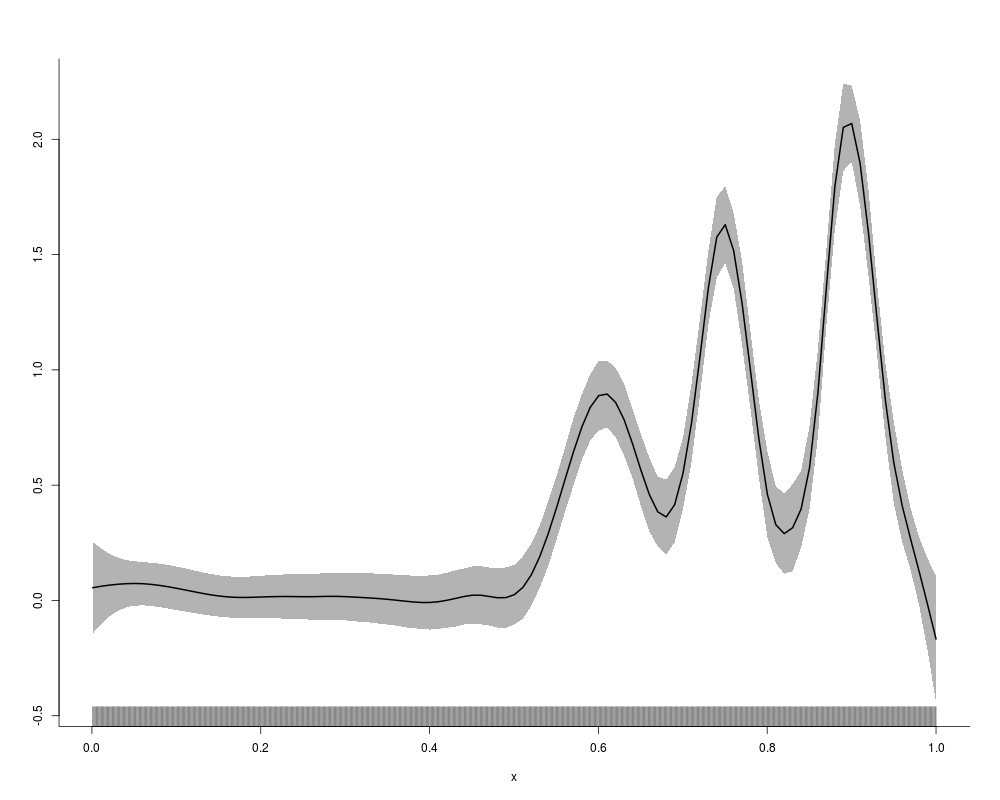
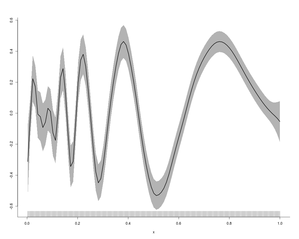
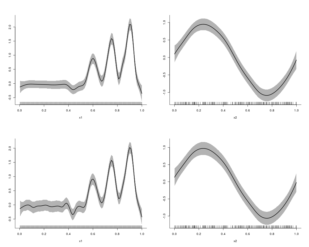
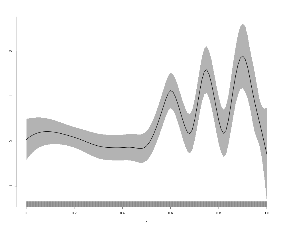
Examples## scatterplot smoothing x <- 1:1000/1000 mu <- exp(-400*(x-0.6)^2)+5*exp(-500*(x-0.75)^2)/3+2*exp(-500*(x-0.9)^2) y <- mu+0.5*rnorm(1000) #fit with default knots y.fit <- asp(y~f(x)) plot(y.fit) ## one more scatterplot smoothing with specified knots and subknots x <- 1:400/400 mu <- sqrt(x*(1-x))*sin((2*pi*(1+2^((9-4*6)/5)))/(x+2^((9-4*6)/5))) y <- mu+0.2*rnorm(400) kn <- default.knots(x,80) kn.var <- default.knots(kn,20) y.fit <- asp(y~f(x,knots=kn,var.knot=kn.var)) plot(y.fit) ## additive models x1 <- 1:300/300 x2 <- runif(300) mu1 <- exp(-400*(x1-0.6)^2)+5*exp(-500*(x1-0.75)^2)/3+2*exp(-500*(x1-0.9)^2) mu2 <- sin(2*pi*x2) y2 <- mu1+mu2+0.3*rnorm(300) y2.fit <- asp(y2~f(x1)+f(x2)) par(mfrow=c(2,2)) y21.fit <- asp(y2~f(x1,adap=FALSE)+f(x2)) #switch off adaptive fitting for the first function plot(y2.fit) plot(y21.fit) par(mfrow=c(1,1)) ## spatial smoothing mu3 <- x1*sin(4*pi*x2) y3 <- mu3+diff(range(mu3))*rnorm(300)/4 #for the specified knots and subknots use # kn <- default.knots.2D(x1,x2,12^2) # !!! interactive function !!! # kn.var <- default.knots.2D(kn[,1],kn[,2],5^2) # y3.fit <- asp(y3~f(x1,x2,knots=kn,var.knot=kn.var)) ## non-normal response x <- 1:1000/1000 mu <- exp(-400*(x-0.6)^2)+5*exp(-500*(x-0.75)^2)/3+2*exp(-500*(x-0.9)^2) y4 <- rbinom(1000,5,1/(1+exp(-mu))) nn <- rep(5,1000) y4.fit <- asp(cbind(y4,nn-y4)~f(x),family="binomial") ### same as ### y4.fit <- asp(y4/nn~f(x),family="binomial",weights=nn) plot(y4.fit) #plot of systematic component ## correlated errors y5 <- sin(2*pi*x1)+0.3*arima.sim(300,model=list(ar=0.6)) y5.fit <- asp(y5~f(x1),adap=FALSE,correlation=corAR1()) plot(y5.fit) #see also SemiPar User Manual # # The current version of the SemiPar User Manual is posted on the web-site: # # www.maths.unsw.edu.au/~wand/papers.html Results
R version 3.3.1 (2016-06-21) -- "Bug in Your Hair"
Copyright (C) 2016 The R Foundation for Statistical Computing
Platform: x86_64-pc-linux-gnu (64-bit)
R is free software and comes with ABSOLUTELY NO WARRANTY.
You are welcome to redistribute it under certain conditions.
Type 'license()' or 'licence()' for distribution details.
R is a collaborative project with many contributors.
Type 'contributors()' for more information and
'citation()' on how to cite R or R packages in publications.
Type 'demo()' for some demos, 'help()' for on-line help, or
'help.start()' for an HTML browser interface to help.
Type 'q()' to quit R.
> library(AdaptFit)
Loading required package: SemiPar
Loading required package: MASS
Loading required package: nlme
Loading required package: cluster
> png(filename="/home/ddbj/snapshot/RGM3/R_CC/result/AdaptFit/asp.Rd_%03d_medium.png", width=480, height=480)
> ### Name: asp
> ### Title: Fit a semiparametric regression model with spatially adaptive
> ### penalized splines
> ### Aliases: asp
> ### Keywords: nonlinear models smooth regression adaptive
>
> ### ** Examples
>
>
> ## scatterplot smoothing
>
> x <- 1:1000/1000
> mu <- exp(-400*(x-0.6)^2)+5*exp(-500*(x-0.75)^2)/3+2*exp(-500*(x-0.9)^2)
> y <- mu+0.5*rnorm(1000)
>
> #fit with default knots
> y.fit <- asp(y~f(x))
> plot(y.fit)
>
> ## one more scatterplot smoothing with specified knots and subknots
>
> x <- 1:400/400
> mu <- sqrt(x*(1-x))*sin((2*pi*(1+2^((9-4*6)/5)))/(x+2^((9-4*6)/5)))
> y <- mu+0.2*rnorm(400)
>
> kn <- default.knots(x,80)
> kn.var <- default.knots(kn,20)
>
> y.fit <- asp(y~f(x,knots=kn,var.knot=kn.var))
> plot(y.fit)
>
>
> ## additive models
>
> x1 <- 1:300/300
> x2 <- runif(300)
> mu1 <- exp(-400*(x1-0.6)^2)+5*exp(-500*(x1-0.75)^2)/3+2*exp(-500*(x1-0.9)^2)
> mu2 <- sin(2*pi*x2)
> y2 <- mu1+mu2+0.3*rnorm(300)
>
> y2.fit <- asp(y2~f(x1)+f(x2))
> par(mfrow=c(2,2))
> y21.fit <- asp(y2~f(x1,adap=FALSE)+f(x2)) #switch off adaptive fitting for the first function
> plot(y2.fit)
> plot(y21.fit)
> par(mfrow=c(1,1))
>
> ## spatial smoothing
>
> mu3 <- x1*sin(4*pi*x2)
> y3 <- mu3+diff(range(mu3))*rnorm(300)/4
>
>
> #for the specified knots and subknots use
> # kn <- default.knots.2D(x1,x2,12^2) # !!! interactive function !!!
> # kn.var <- default.knots.2D(kn[,1],kn[,2],5^2)
> # y3.fit <- asp(y3~f(x1,x2,knots=kn,var.knot=kn.var))
>
> ## non-normal response
>
> x <- 1:1000/1000
> mu <- exp(-400*(x-0.6)^2)+5*exp(-500*(x-0.75)^2)/3+2*exp(-500*(x-0.9)^2)
> y4 <- rbinom(1000,5,1/(1+exp(-mu)))
> nn <- rep(5,1000)
> y4.fit <- asp(cbind(y4,nn-y4)~f(x),family="binomial")
iteration 1
iteration 2
iteration 3
iteration 1
iteration 2
iteration 3
iteration 4
iteration 1
iteration 2
iteration 3
iteration 4
iteration 1
iteration 2
iteration 3
iteration 4
iteration 1
iteration 2
iteration 3
iteration 4
> ### same as ### y4.fit <- asp(y4/nn~f(x),family="binomial",weights=nn)
> plot(y4.fit) #plot of systematic component
>
>
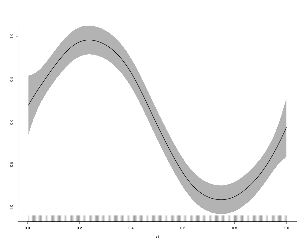
> ## correlated errors
>
> y5 <- sin(2*pi*x1)+0.3*arima.sim(300,model=list(ar=0.6))
>
> y5.fit <- asp(y5~f(x1),adap=FALSE,correlation=corAR1())
> plot(y5.fit)
>
> #see also SemiPar User Manual
>
> #
> # The current version of the SemiPar User Manual is posted on the web-site:
> #
> # www.maths.unsw.edu.au/~wand/papers.html
>
>
>
>
>
> dev.off()
null device
1
>
|