R Graphical Manual

Browse All

Last data update: 2014.03.03

R: Fit a semiparametric regression model with spatially adaptive...

asp2	R Documentation

Fit a semiparametric regression model with spatially adaptive penalized splines

Description

Fits semiparametric regression models using the mixed model representation of penalized splines with spatially adaptive penalties based on the asp function from package AdaptFit. Particular differences to AdaptFit include the availability of simultaneous confidence bands and B-spline basis functions and different functionality of the plot function. However, random effects, autocorrelations and interaction surfaces are not supported. Further, only Gaussian responses are supported. Note that in contrast to AdaptFit, estimated curves are centered to have zero mean.

Usage

asp2(form, spar.method = "REML", contrasts=NULL, 
     omit.missing = NULL, returnFit=FALSE, 
     niter = 20, niter.var = 50, tol=1e-6, tol.theta=1e-6, 
     control=NULL)

Arguments

form

a formula describing the model to be fitted. See aspFormula for further information. Note, that an intercept is always included, whether given in the formula or not.

`spar.method`	method for automatic smoothing parameter selection. May be "REML" (restricted maximum likelihood) or "ML" (maximum likelihood).
`contrasts`	an optional list. See the `contrasts.arg` of `model.matrix.default`.
`omit.missing`	a logical value indicating whether fields with missing values are to be omitted.
`niter`	a maximum number of iterations for the mean estimation, default is 20.
`niter.var`	a maximum number of iterations for the variance of random effects estimation, default is 50.
`tol`	tolerance for the convergence criterion. Default is 1e-6.
`tol.theta`	tolerance for the convergence criterion (smoothing parameter function routine). Default is 1e-6.
`returnFit`	a logical value indicating whether the fitted object should be returned when the maximum number of iterations is reached without convergence of the algorithm. Default is FALSE.
`control`	see lmeControl in the documentation to `nlme`.

Value

A list object of class asp containing the fitted model. The components are:

`fitted`	fitted values.
`coef.mean`	estimated mean coefficients.
`design.matrices`	design matrices both for knots und subknots.
`x`	x values.
`knots`	knots.
`y.cov`	estimated covariance matrix of the response.
`random.var`	estimated covariance matrix of the random effects.
`subknots`	subknots.
`coef.random`	estimated spline coefficients of the covariance matrix of the random effects.
`var.random.var`	estimated variance of the spline coefficients of the covariance matrix of the random effects.
`fit`	mimics fit object of lme().
`info`	information about the inputs.
`aux`	auxiliary information such as variability estimates.

Author(s)

Manuel Wiesenfarth m.wiesenfarth at dkfz de, Tatyana Krivobokova tkrivob at gwdg.de

References

Krivobokova, T., Crainiceanu, C.M. and Kauermann, G. (2008)
Fast Adaptive Penalized Splines. Journal of Computational and Graphical Statistics. 17(1) 1-20.

Ruppert, D., Wand, M.P. and Carroll, R.J. (2003)
Semiparametric Regression Cambridge University Press.
http://stat.tamu.edu/~carroll/semiregbook/

Wiesenfarth, M., Krivobokova, T., Klasen, S., Sperlich, S. (2012).
Direct Simultaneous Inference in Additive Models and its Application to Model Undernutrition. Journal of the American Statistical Association, 107(500): 1286-1296.

Examples

############
# Examples as in package AdaptFit
  ## scatterplot smoothing
    x <- 1:1000/1000
    mu <- exp(-400*(x-0.6)^2)+
    			5*exp(-500*(x-0.75)^2)/3+2*exp(-500*(x-0.9)^2)
    y <- mu+0.5*rnorm(1000)

  #fit with default knots
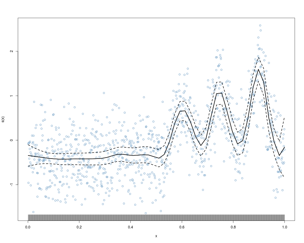
    y.fit <- asp2(y~f(x,adap=TRUE))
    plot(y.fit,residuals=TRUE,lwd=2,scb.lwd=2,scb.lty="dashed")
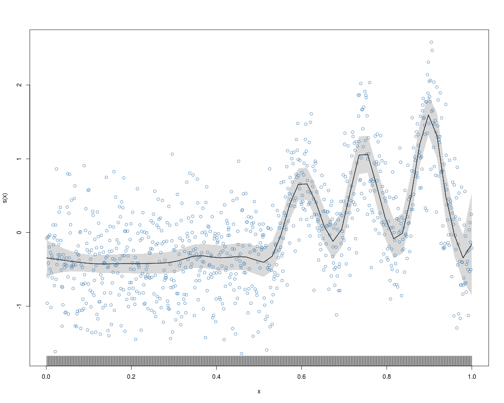
    # with shaded confidence region. 
    # Use scb.lty="blank" to plot the shades only.
      plot(y.fit,residuals=TRUE,shade=TRUE,scb.lty="blank")

 ## Not run: 
 ## additive models
    x1 <- 1:300/300
    x2 <- runif(300)
    mu1 <- exp(-400*(x1-0.6)^2)+
    			 5*exp(-500*(x1-0.75)^2)/3+2*exp(-500*(x1-0.9)^2)
    mu2 <- sin(2*pi*x2)
    y2 <- mu1+mu2+0.3*rnorm(300)

    y2.fit <- asp2(y2~f(x1,adap=TRUE)+f(x2,adap=TRUE))
    # switch off adaptive fitting for the first function
      y21.fit <- asp2(y2~f(x1,adap=FALSE)+f(x2,adap=TRUE))
    op <- par(mfrow = c(2, 2))
    plot(y2.fit)
    plot(y21.fit)
    par(op)


  ## scatterplot smoothing with specified knots and subknots
    x <- 1:400/400
    mu <- sqrt(x*(1-x))*sin((2*pi*(1+2^((9-4*6)/5)))/(x+2^((9-4*6)/5)))
    y <- mu+0.2*rnorm(400)

    kn <- default.knots(x,80)
    kn.var <- default.knots(kn,20)

    y.fit <- asp2(y~f(x,knots=kn))
    y.fit2 <- asp2(y~f(x,knots=kn,var.knots=kn.var,adap=TRUE))
    op <- par(mfrow = c(1, 2))
    plot(y.fit)
    plot(y.fit2)
    par(op)

##################
#more examples
  beta=function(l,m,x) 
  		return(gamma(l+m)*(gamma(l)*gamma(m))^(-1)*x^(l-1)*(1-x)^(m-1))
  f1 = function(x) return((0.6*beta(30,17,x)+0.4*beta(3,11,x))*1/0.958)
  f2 = function(z) return((sin(2*pi*(z-0.5))^2)*1/.3535)
  f3 = function(z) 
  		return((exp(-400*(z-0.6)^2)+
  				5/3*exp(-500*(z-0.75)^2)+2*exp(-500*(z-0.9)^2))*1/0.549)

  set.seed(1)
  N <- 500
  x1 = runif(N,0,1)
  x2 = runif(N,0,1)
  x3 = runif(N,0,1)


  kn1 <- default.knots(x1,40)
  kn2 <- default.knots(x2,40)
  kn3 <- default.knots(x3,40)
  kn.var3 <- default.knots(kn3,5)

  y <- f1(x1)+f2(x2)+f3(x3)+0.3*rnorm(N)

  # semiparametric model
    fit1=  asp2(y~x1+f(x2,basis="os",degree=3,knots=kn2,adap=FALSE)
                    +f(x3,basis="os",degree=3,
                    	   knots=kn3,var.knots=kn.var3,adap=FALSE),
                    niter = 20, niter.var = 200)
    summary(fit1)
    plot(fit1,pages=1)


  # all effects flexible
  # fit model with all smoothing parameters constant
    fit2a= asp2(y~f(x1,basis="os",degree=3,knots=kn1,adap=FALSE)
                  +f(x2,basis="os",degree=3,knots=kn2,adap=FALSE)
                  +f(x3,basis="os",degree=3,knots=kn3,adap=FALSE),
                  niter = 20, niter.var = 200)
    plot(fit2a,pages=1)

  # fit model with last smoothing parameter adaptive
    fit2b= asp2(y~f(x1,basis="os",degree=3,knots=kn1,adap=FALSE)
                  +f(x2,basis="os",degree=3,knots=kn2,adap=FALSE)
                  +f(x3,basis="os",degree=3,knots=kn3,adap=TRUE,
                     var.knots=kn.var3,var.basis="os",var.degree=3),
                 niter = 20, niter.var = 200)

  # plot smoothing parameter function for covariate x3.
  # Note that in the case of B-splines additional knots are added, 
  # see references.
    plot(seq(0,1,length.out=42), fit2b$y.cov/fit2b$random.var[85:126],
                ylab=expression(lambda(x3)),xlab="x3",type="l",lwd=3)

  # compute 95
  # You could skip this and use "fit2b" indstead of "scb2b" later on, however,
  # if N is large, computing the SCBs various times can take some time
  # if you don't need fitted values and bounds for all covariate points
  # (can be computationally intensive due to large matrix dimensions),
  # set calc.stdev=F such that these are not computed.
    scb2b<- scbM(fit2b,calc.stdev=FALSE)
    plot(scb2b,pages=1)

  # plot only f(x2).
    plot(scb2b,select=2,mfrow=c(1,1),lwd=3,ylab="f(x2)",xlab="x2")
  # plot.scbm (and plot.asp) returns fitted values and confidence limits,
  # if you only need the returned object set plot=FALSE
    pscb=plot(scb2b,plot=FALSE)
  # add pointwise confidence intervals to the plot
    polygon(c(pscb$grid.x[[2]], rev(pscb$grid.x[[2]])),
            c(pscb$fitted[[2]]+1.96*pscb$Stdev[[2]],
              rev(pscb$fitted[[2]]-1.96*pscb$Stdev[[2]])),
            col = grey(0.85), border = NA)
    lines(pscb$grid.x[[2]],pscb$lcb[[2]],lty="dotted",lwd=3)
    lines(pscb$grid.x[[2]],pscb$fitted[[2]],lwd=3)
    lines(pscb$grid.x[[2]],pscb$ucb[[2]],lty="dotted",lwd=3)

  # plot first derivative of f(x1)
    scb2bdrv<- scbM(fit2b,drv=1,calc.stdev=FALSE)
    plot(scb2bdrv,select=1)
    #the following would give the same result
    #x11();plot(fit2b,select=1,drv=1)
  # different style
    plot(scb2bdrv,select=1,scb.lty="blank", 
    				shade=TRUE,shade.col="steelblue")

## End(Not run)

Results


R version 3.3.1 (2016-06-21) -- "Bug in Your Hair"
Copyright (C) 2016 The R Foundation for Statistical Computing
Platform: x86_64-pc-linux-gnu (64-bit)

R is free software and comes with ABSOLUTELY NO WARRANTY.
You are welcome to redistribute it under certain conditions.
Type 'license()' or 'licence()' for distribution details.

R is a collaborative project with many contributors.
Type 'contributors()' for more information and
'citation()' on how to cite R or R packages in publications.

Type 'demo()' for some demos, 'help()' for on-line help, or
'help.start()' for an HTML browser interface to help.
Type 'q()' to quit R.

> library(AdaptFitOS)
Loading required package: nlme
Loading required package: MASS
Loading required package: splines

AdaptFitOS 0.62 loaded. Type 'help("AdaptFitOS-package")' for an overview.

Please cite as:
   Wiesenfarth, M., Krivobokova, T., Klasen, S., & Sperlich, S. (2012).
   Direct simultaneous inference in additive models and its application to model undernutrition.
   Journal of the American Statistical Association, 107(500), 1286-1296.

Attaching package: 'AdaptFitOS'

The following object is masked from 'package:stats':

    sigma

> png(filename="/home/ddbj/snapshot/RGM3/R_CC/result/AdaptFitOS/asp2.Rd_%03d_medium.png", width=480, height=480)
> ### Name: asp2
> ### Title: Fit a semiparametric regression model with spatially adaptive
> ###   penalized splines
> ### Aliases: asp2
> ### Keywords: nonlinear models smooth regression adaptive
> 
> ### ** Examples
> 
> ############
> # Examples as in package AdaptFit
>   ## scatterplot smoothing
>     x <- 1:1000/1000
>     mu <- exp(-400*(x-0.6)^2)+
+     			5*exp(-500*(x-0.75)^2)/3+2*exp(-500*(x-0.9)^2)
>     y <- mu+0.5*rnorm(1000)
> 
>   #fit with default knots
>     y.fit <- asp2(y~f(x,adap=TRUE))
>     plot(y.fit,residuals=TRUE,lwd=2,scb.lwd=2,scb.lty="dashed")
Critical value for f(x): 3.423244
>     # with shaded confidence region. 
>     # Use scb.lty="blank" to plot the shades only.
>       plot(y.fit,residuals=TRUE,shade=TRUE,scb.lty="blank")
Critical value for f(x): 3.423244
> 
>  ## Not run: 
> ##D  ## additive models
> ##D     x1 <- 1:300/300
> ##D     x2 <- runif(300)
> ##D     mu1 <- exp(-400*(x1-0.6)^2)+
> ##D     			 5*exp(-500*(x1-0.75)^2)/3+2*exp(-500*(x1-0.9)^2)
> ##D     mu2 <- sin(2*pi*x2)
> ##D     y2 <- mu1+mu2+0.3*rnorm(300)
> ##D 
> ##D     y2.fit <- asp2(y2~f(x1,adap=TRUE)+f(x2,adap=TRUE))
> ##D     # switch off adaptive fitting for the first function
> ##D       y21.fit <- asp2(y2~f(x1,adap=FALSE)+f(x2,adap=TRUE))
> ##D     op <- par(mfrow = c(2, 2))
> ##D     plot(y2.fit)
> ##D     plot(y21.fit)
> ##D     par(op)
> ##D 
> ##D 
> ##D   ## scatterplot smoothing with specified knots and subknots
> ##D     x <- 1:400/400
> ##D     mu <- sqrt(x*(1-x))*sin((2*pi*(1+2^((9-4*6)/5)))/(x+2^((9-4*6)/5)))
> ##D     y <- mu+0.2*rnorm(400)
> ##D 
> ##D     kn <- default.knots(x,80)
> ##D     kn.var <- default.knots(kn,20)
> ##D 
> ##D     y.fit <- asp2(y~f(x,knots=kn))
> ##D     y.fit2 <- asp2(y~f(x,knots=kn,var.knots=kn.var,adap=TRUE))
> ##D     op <- par(mfrow = c(1, 2))
> ##D     plot(y.fit)
> ##D     plot(y.fit2)
> ##D     par(op)
> ##D 
> ##D ##################
> ##D #more examples
> ##D   beta=function(l,m,x) 
> ##D   		return(gamma(l+m)*(gamma(l)*gamma(m))^(-1)*x^(l-1)*(1-x)^(m-1))
> ##D   f1 = function(x) return((0.6*beta(30,17,x)+0.4*beta(3,11,x))*1/0.958)
> ##D   f2 = function(z) return((sin(2*pi*(z-0.5))^2)*1/.3535)
> ##D   f3 = function(z) 
> ##D   		return((exp(-400*(z-0.6)^2)+
> ##D   				5/3*exp(-500*(z-0.75)^2)+2*exp(-500*(z-0.9)^2))*1/0.549)
> ##D 
> ##D   set.seed(1)
> ##D   N <- 500
> ##D   x1 = runif(N,0,1)
> ##D   x2 = runif(N,0,1)
> ##D   x3 = runif(N,0,1)
> ##D 
> ##D 
> ##D   kn1 <- default.knots(x1,40)
> ##D   kn2 <- default.knots(x2,40)
> ##D   kn3 <- default.knots(x3,40)
> ##D   kn.var3 <- default.knots(kn3,5)
> ##D 
> ##D   y <- f1(x1)+f2(x2)+f3(x3)+0.3*rnorm(N)
> ##D 
> ##D   # semiparametric model
> ##D     fit1=  asp2(y~x1+f(x2,basis="os",degree=3,knots=kn2,adap=FALSE)
> ##D                     +f(x3,basis="os",degree=3,
> ##D                     	   knots=kn3,var.knots=kn.var3,adap=FALSE),
> ##D                     niter = 20, niter.var = 200)
> ##D     summary(fit1)
> ##D     plot(fit1,pages=1)
> ##D 
> ##D 
> ##D   # all effects flexible
> ##D   # fit model with all smoothing parameters constant
> ##D     fit2a= asp2(y~f(x1,basis="os",degree=3,knots=kn1,adap=FALSE)
> ##D                   +f(x2,basis="os",degree=3,knots=kn2,adap=FALSE)
> ##D                   +f(x3,basis="os",degree=3,knots=kn3,adap=FALSE),
> ##D                   niter = 20, niter.var = 200)
> ##D     plot(fit2a,pages=1)
> ##D 
> ##D   # fit model with last smoothing parameter adaptive
> ##D     fit2b= asp2(y~f(x1,basis="os",degree=3,knots=kn1,adap=FALSE)
> ##D                   +f(x2,basis="os",degree=3,knots=kn2,adap=FALSE)
> ##D                   +f(x3,basis="os",degree=3,knots=kn3,adap=TRUE,
> ##D                      var.knots=kn.var3,var.basis="os",var.degree=3),
> ##D                  niter = 20, niter.var = 200)
> ##D 
> ##D   # plot smoothing parameter function for covariate x3.
> ##D   # Note that in the case of B-splines additional knots are added, 
> ##D   # see references.
> ##D     plot(seq(0,1,length.out=42), fit2b$y.cov/fit2b$random.var[85:126],
> ##D                 ylab=expression(lambda(x3)),xlab="x3",type="l",lwd=3)
> ##D 
> ##D   # compute 95##D 
> ##D   # You could skip this and use "fit2b" indstead of "scb2b" later on, however,
> ##D   # if N is large, computing the SCBs various times can take some time
> ##D   # if you don't need fitted values and bounds for all covariate points
> ##D   # (can be computationally intensive due to large matrix dimensions),
> ##D   # set calc.stdev=F such that these are not computed.
> ##D     scb2b<- scbM(fit2b,calc.stdev=FALSE)
> ##D     plot(scb2b,pages=1)
> ##D 
> ##D   # plot only f(x2).
> ##D     plot(scb2b,select=2,mfrow=c(1,1),lwd=3,ylab="f(x2)",xlab="x2")
> ##D   # plot.scbm (and plot.asp) returns fitted values and confidence limits,
> ##D   # if you only need the returned object set plot=FALSE
> ##D     pscb=plot(scb2b,plot=FALSE)
> ##D   # add pointwise confidence intervals to the plot
> ##D     polygon(c(pscb$grid.x[[2]], rev(pscb$grid.x[[2]])),
> ##D             c(pscb$fitted[[2]]+1.96*pscb$Stdev[[2]],
> ##D               rev(pscb$fitted[[2]]-1.96*pscb$Stdev[[2]])),
> ##D             col = grey(0.85), border = NA)
> ##D     lines(pscb$grid.x[[2]],pscb$lcb[[2]],lty="dotted",lwd=3)
> ##D     lines(pscb$grid.x[[2]],pscb$fitted[[2]],lwd=3)
> ##D     lines(pscb$grid.x[[2]],pscb$ucb[[2]],lty="dotted",lwd=3)
> ##D 
> ##D   # plot first derivative of f(x1)
> ##D     scb2bdrv<- scbM(fit2b,drv=1,calc.stdev=FALSE)
> ##D     plot(scb2bdrv,select=1)
> ##D     #the following would give the same result
> ##D     #x11();plot(fit2b,select=1,drv=1)
> ##D   # different style
> ##D     plot(scb2bdrv,select=1,scb.lty="blank", 
> ##D     				shade=TRUE,shade.col="steelblue")
> ## End(Not run)
> 
> 
> 
> 
> 
> dev.off()
null device 
          1 
>