R Graphical Manual

Browse All

Last data update: 2014.03.03

R: Estimate varying residual variance

aspHetero

R Documentation

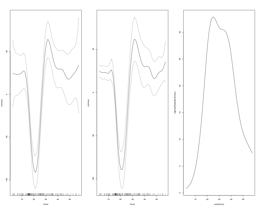
Estimate varying residual variance

Description

Estimates a varying residual variance on basis of an asp object.

Usage

aspHetero(object, xx, nknots=5, knots=NULL, basis="os", 
		 degree=c(3,2), tol=1e-8, niter=100, niter.var=250)

Arguments

`object`	an asp object.
`xx`	the covariate.
`nknots`	the number of knots. Does not apply when `knots` are given.
`knots`	the knots. Does not apply if basis=="os". Otherwise, if `NULL` `nknots` equidistant knots are used.
`basis`	the spline basis: "os" (default), "trunc.poly" or "tps".
`degree`	the spline degree (and penalty order in case of B-splines). Defaults to c(3,2).
`tol`	tolerance for the convergence criterion. Default is 1e-8.
`niter`	a maximum number of iterations for residual variance function estimation, default is 100.
`niter.var`	a maximum number of iterations for the variance of random effects estimation within the residual variance function estimation routine, default is 250.

Value

An object of class asp with varying variances, with additional element sigmax including information on the spline of the varying variance.

Author(s)

Manuel Wiesenfarth m.wiesenfarth at dkfz de

References

Wiesenfarth, M., Krivobokova, T., Klasen, S., Sperlich, S. (2012).
Direct Simultaneous Inference in Additive Models and its Application to Model Undernutrition. Journal of the American Statistical Association, 107(500): 1286-1296.

Examples

#dontrun{
attach(mcycle)

y=accel
kn1 <- default.knots(times,20)
# fit model with constant residual variance
  fit= asp2(accel~f(times,basis="os",degree=3,knots=kn1,adap=FALSE),
  								niter = 20, niter.var = 200)


# fit model with varying residual variance
fith=aspHetero(fit,times,tol=1e-8)
op <- par(mfrow = c(1,3))
plot(fit);plot(fith)
#sigma() returns the fitted varying residual variance
plot(sort(times),sigma(fith)[order(times)],type="l")
par(op)
#}

Results


R version 3.3.1 (2016-06-21) -- "Bug in Your Hair"
Copyright (C) 2016 The R Foundation for Statistical Computing
Platform: x86_64-pc-linux-gnu (64-bit)

R is free software and comes with ABSOLUTELY NO WARRANTY.
You are welcome to redistribute it under certain conditions.
Type 'license()' or 'licence()' for distribution details.

R is a collaborative project with many contributors.
Type 'contributors()' for more information and
'citation()' on how to cite R or R packages in publications.

Type 'demo()' for some demos, 'help()' for on-line help, or
'help.start()' for an HTML browser interface to help.
Type 'q()' to quit R.

> library(AdaptFitOS)
Loading required package: nlme
Loading required package: MASS
Loading required package: splines

AdaptFitOS 0.62 loaded. Type 'help("AdaptFitOS-package")' for an overview.

Please cite as:
   Wiesenfarth, M., Krivobokova, T., Klasen, S., & Sperlich, S. (2012).
   Direct simultaneous inference in additive models and its application to model undernutrition.
   Journal of the American Statistical Association, 107(500), 1286-1296.

Attaching package: 'AdaptFitOS'

The following object is masked from 'package:stats':

    sigma

> png(filename="/home/ddbj/snapshot/RGM3/R_CC/result/AdaptFitOS/aspHetero.Rd_%03d_medium.png", width=480, height=480)
> ### Name: aspHetero
> ### Title: Estimate varying residual variance
> ### Aliases: aspHetero
> ### Keywords: smooth
> 
> ### ** Examples
> 
> #dontrun{
> attach(mcycle)
> 
> y=accel
> kn1 <- default.knots(times,20)
> # fit model with constant residual variance
>   fit= asp2(accel~f(times,basis="os",degree=3,knots=kn1,adap=FALSE),
+   								niter = 20, niter.var = 200)
> 
> 
> # fit model with varying residual variance
> fith=aspHetero(fit,times,tol=1e-8)
> op <- par(mfrow = c(1,3))
> plot(fit);plot(fith)
Critical value for f(times): 3.315361
Critical value for f(times): 3.371649
> #sigma() returns the fitted varying residual variance
> plot(sort(times),sigma(fith)[order(times)],type="l")
> par(op)
> #}
> 
> 
> 
> 
> 
> dev.off()
null device 
          1 
>