Supported by Dr. Osamu Ogasawara and  . . |
|
Last data update: 2014.03.03 |
Adequacy of modelsDescriptionThis function provides some useful statistics to assess the quality of fit of probabilistic models, including the statistics Cramér-von Mises and Anderson-Darling. These statistics are often used to compare models not fitted. You can also calculate other goodness of fit such as AIC, CAIC, BIC, HQIC and Kolmogorov-Smirnov test. Usage
goodness.fit(pdf, cdf, starts, data, method = "PSO", domain = c(0,Inf),
             mle = NULL,...)
Arguments
DetailsThe function The Kolmogorov-Smirnov test may return By default, the function calculates the maximum likelihood estimates. The errors of the estimates are also calculated. In cases that the function can not obtain the maximum likelihood estimates, the change of the values initial, in some cases, resolve the problem. You can also enter with the maximum likelihood estimation if there is already prior knowledge. Value
NoteIt is not necessary to define the likelihood function or log-likelihood. You only need to define the probability density function and distribution function. Author(s)Pedro Rafael Diniz Marinho pedro.rafael.marinho@gmail.com ReferencesChen, G., Balakrishnan, N. (1995). A general purpose approximate goodness-of-fit test. Journal of Quality Technology, 27, 154-161. Hannan, E. J. and Quinn, B. G. (1979). The Determination of the Order of an Autoregression. Journal of the Royal Statistical Society, Series B, 41, 190-195. Nocedal, J. and Wright, S. J. (1999) Numerical Optimization. Springer. Sakamoto, Y., Ishiguro, M. and Kitagawa G. (1986). Akaike Information Criterion Statistics. D. Reidel Publishing Company. See AlsoFor details about the optimization methodologies may view the functions Examples
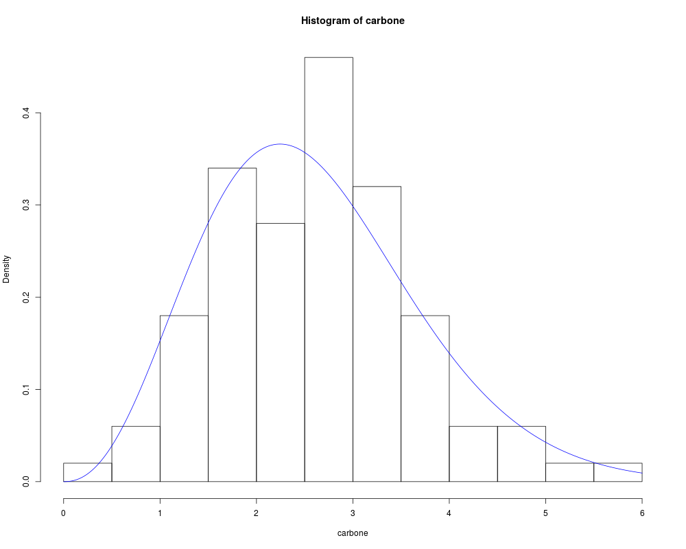
# Example 1:
data(carbone)
# Exponentiated Weibull - Probability density function.
pdf_expweibull <- function(par,x){
beta = par[1]
c = par[2]
a = par[3]
a * beta * c * exp(-(beta*x)^c) * (beta*x)^(c-1) * (1 - exp(-(beta*x)^c))^(a-1)
}
# Exponentiated Weibull - Cumulative distribution function.
cdf_expweibull <- function(par,x){
beta = par[1]
c = par[2]
a = par[3]
(1 - exp(-(beta*x)^c))^a
}
set.seed(0)
result_1 = goodness.fit(pdf = pdf_expweibull, cdf = cdf_expweibull,
starts = c(1,1,1), data = carbone, method = "PSO",
domain = c(0,Inf),mle = NULL, lim_inf = c(0,0,0),
lim_sup = c(2,2,2), S = 250, prop=0.1, N=50)
x = seq(0, 6, length.out = 500)
hist(carbone, probability = TRUE)
lines(x, pdf_expweibull(x, par = result_1$mle), col = "blue")
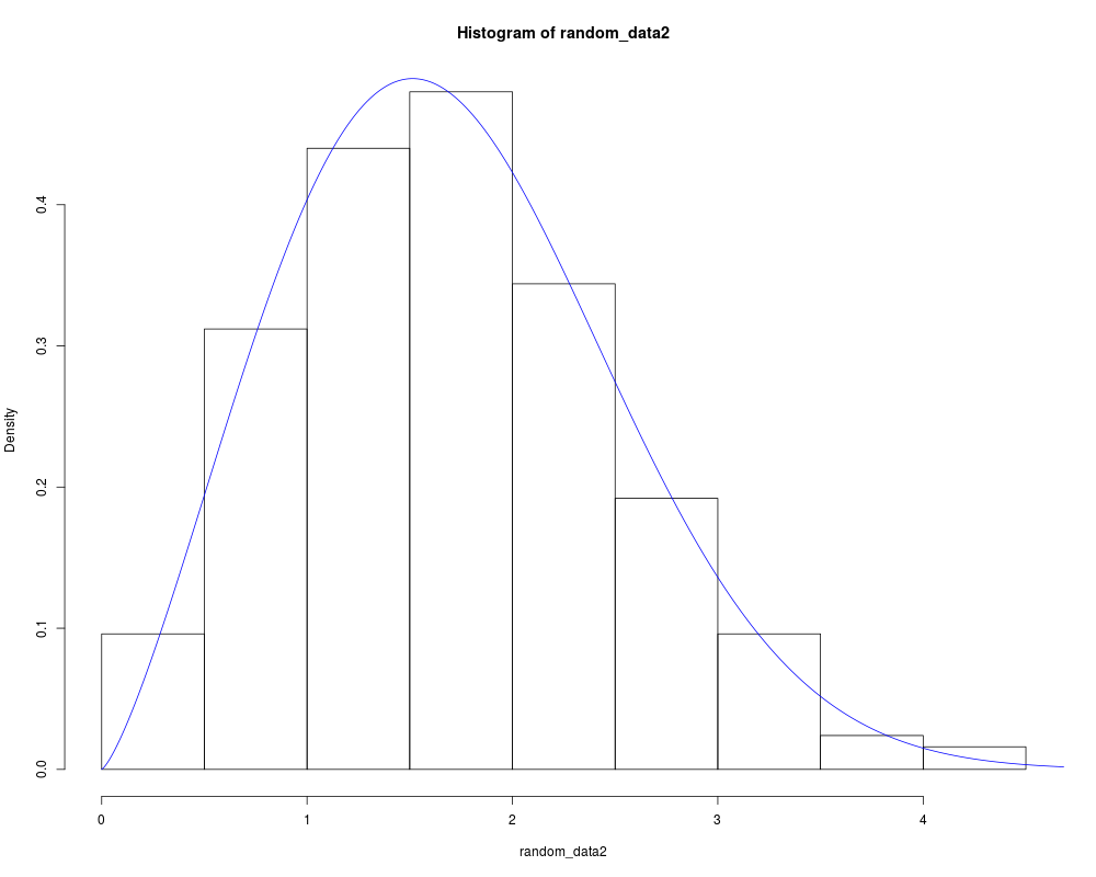
# Example 2:
pdf_weibull <- function(par,x){
a = par[1]
b = par[2]
dweibull(x, shape = a, scale = b)
}
cdf_weibull <- function(par,x){
a = par[1]
b = par[2]
pweibull(x, shape = a, scale = b)
}
set.seed(0)
random_data2 = rweibull(250,2,2)
result_2 = goodness.fit(pdf = pdf_weibull, cdf = cdf_weibull, starts = c(1,1), data = random_data2,
method = "PSO", domain = c(0,Inf), mle = NULL, lim_inf = c(0,0), lim_sup = c(10,10),
N = 100, S = 250)
x = seq(0,ceiling(max(random_data2)), length.out = 500)
hist(random_data2, probability = TRUE)
lines(x, pdf_weibull(par = result_2$mle, x), col = "blue")
# TO RUN THE CODE BELOW, UNCOMMENT THE CODES.
# Example 3:
# Kumaraswamy Beta - Probability density function.
#pdf_kwbeta <- function(par,x){
# beta = par[1]
# a = par[2]
# alpha = par[3]
# b = par[4]
# (a*b*x^(alpha-1)*(1-x)^(beta-1)*(pbeta(x,alpha,beta))^(a-1)*
# (1-pbeta(x,alpha,beta)^a)^(b-1))/beta(alpha,beta)
#}
# Kumaraswamy Beta - Cumulative distribution function.
#cdf_kwbeta <- function(par,x){
# beta = par[1]
# a = par[2]
# alpha = par[3]
# b = par[4]
# 1 - (1 - pbeta(x,alpha,beta)^a)^b
#}
#set.seed(0)
#random_data3 = rbeta(150,2,2.2)
#system.time(goodness.fit(pdf = pdf_kwbeta, cdf = cdf_kwbeta, starts = c(1,1,1,1),
# data = random_data3, method = "PSO", domain = c(0,1), lim_inf = c(0,0,0,0),
# lim_sup = c(10,10,10,10), S = 200, prop = 0.1, N = 40))
Results
R version 3.3.1 (2016-06-21) -- "Bug in Your Hair"
Copyright (C) 2016 The R Foundation for Statistical Computing
Platform: x86_64-pc-linux-gnu (64-bit)

R is free software and comes with ABSOLUTELY NO WARRANTY.
You are welcome to redistribute it under certain conditions.
Type 'license()' or 'licence()' for distribution details.

R is a collaborative project with many contributors.
Type 'contributors()' for more information and
'citation()' on how to cite R or R packages in publications.

Type 'demo()' for some demos, 'help()' for on-line help, or
'help.start()' for an HTML browser interface to help.
Type 'q()' to quit R.

> library(AdequacyModel)
> png(filename="/home/ddbj/snapshot/RGM3/R_CC/result/AdequacyModel/goodness.fit.Rd_%03d_medium.png", width=480, height=480)
> ### Name: goodness.fit
> ### Title: Adequacy of models
> ### Aliases: goodness.fit
> ### Keywords: AdequacyModel pso AIC BIC CAIC distribution survival
>
> ### ** Examples
>
>
> # Example 1:
>
> data(carbone)
>
> # Exponentiated Weibull - Probability density function.
> pdf_expweibull <- function(par,x){
+   beta = par[1]
+   c = par[2]
+   a = par[3]
+   a * beta * c * exp(-(beta*x)^c) * (beta*x)^(c-1) * (1 - exp(-(beta*x)^c))^(a-1)
+ }
>
> # Exponentiated Weibull - Cumulative distribution function.
> cdf_expweibull <- function(par,x){
+   beta = par[1]
+   c = par[2]
+   a = par[3]
+   (1 - exp(-(beta*x)^c))^a
+ }
>
> set.seed(0)
> result_1 = goodness.fit(pdf = pdf_expweibull, cdf = cdf_expweibull,
+                         starts = c(1,1,1), data = carbone, method = "PSO",
+                         domain = c(0,Inf),mle = NULL, lim_inf = c(0,0,0),
+                         lim_sup = c(2,2,2), S = 250, prop=0.1, N=50)
There were 35 warnings (use warnings() to see them)
>
> x = seq(0, 6, length.out = 500)
> hist(carbone, probability = TRUE)
> lines(x, pdf_expweibull(x, par = result_1$mle), col = "blue")
>
> # Example 2:
>
> pdf_weibull <- function(par,x){
+   a = par[1]
+   b = par[2]
+   dweibull(x, shape = a, scale = b)
+ }
>
> cdf_weibull <- function(par,x){
+   a = par[1]
+   b = par[2]
+   pweibull(x, shape = a, scale = b)
+ }
>
> set.seed(0)
> random_data2 = rweibull(250,2,2)
> result_2 = goodness.fit(pdf = pdf_weibull, cdf = cdf_weibull, starts = c(1,1), data = random_data2,
+              method = "PSO", domain = c(0,Inf), mle = NULL, lim_inf = c(0,0), lim_sup = c(10,10),
+              N = 100, S = 250)
There were 50 or more warnings (use warnings() to see the first 50)
>
> x = seq(0,ceiling(max(random_data2)), length.out = 500)
> hist(random_data2, probability = TRUE)
> lines(x, pdf_weibull(par = result_2$mle, x), col = "blue")
>
> # TO RUN THE CODE BELOW, UNCOMMENT THE CODES.
>
> # Example 3:
>
> # Kumaraswamy Beta - Probability density function.
> #pdf_kwbeta <- function(par,x){
> #  beta = par[1]
> #  a = par[2]
> #  alpha = par[3]
> #  b = par[4]
> #  (a*b*x^(alpha-1)*(1-x)^(beta-1)*(pbeta(x,alpha,beta))^(a-1)*
> #  (1-pbeta(x,alpha,beta)^a)^(b-1))/beta(alpha,beta)
> #}
>
> # Kumaraswamy Beta - Cumulative distribution function.
> #cdf_kwbeta <- function(par,x){
> #  beta = par[1]
> #  a = par[2]
> #  alpha = par[3]
> #  b = par[4]
> #  1 - (1 - pbeta(x,alpha,beta)^a)^b
> #}
>
> #set.seed(0)
> #random_data3 = rbeta(150,2,2.2)
>
> #system.time(goodness.fit(pdf = pdf_kwbeta, cdf = cdf_kwbeta, starts = c(1,1,1,1),
> #              data = random_data3, method = "PSO", domain = c(0,1), lim_inf = c(0,0,0,0),
> #              lim_sup = c(10,10,10,10), S = 200, prop = 0.1, N = 40))
>
>
>
>
>
>
>
> dev.off()
null device
          1
>
|