Sexpr[results=rd,stage=build]{tools:::Rd_package_title("AnalyzeTS")}

Description

Details

This package contains 17 functions which are used to analyze time series and 3 data time series.

av.res function: The main function measures the accuracy of forecasted models.

Descriptives function: The main function descriptive statistics of a Time Series, a continous variable or continous variables in a data frame.

Dgroup function: The main function descriptive statistics in group for a continous variable.

forecastGARCH function: The main function extracts the forecast of next day of ARCH or GARCH models.

Frequencies function: The main function descriptive statistics for a desultory variable or desultory variables in a data frame.

fuzzy.ts1 function: The main function calculates fuzziness of time series with Chen, Singh, Heuristic and Chen-Hsu models.

fuzzy.ts2 function: The main function predicts time series by fuzziness method according to Abbasov-Manedova model.

fuzzy.ts3 function: The main function predicts time series by fuzziness method according to Improve Abbasov-Manedova version 1 model.

grid.on function: The main function using to draw grid for line graph ( graph of time series) that is drawn by plot(), ts.plot or plot.ts() function.

PrintAIC function: The main function calculates and outputs AIC value for some models including ARMA, ARIMA, SARIMA, ARMAX, ARIMAX, SARIMAX, ARCH and GARCH.

SES function: The main function calculate simple exponential smoothing for a time series.

CMA function: The main function uses calculating center moving average for a time series

Abbasov.Cs2 function: The main function use to compare and sort Abbasov-Mamedova models according ME, MAE, MPE, MAPE, MSE RMSE for C values in Cs.

Abbasov.Cs3 function: The main function use to comparing and sort Improve Abbasov-Mamedova version 1 models according ME, MAE, MPE, MAPE, MSE RMSE for C values in Cs.

ChenHsu.bin function: The main function use to calculating bin point values, which devece divide fuzzy sets in Chen-Hsu model.

FindC2 function: The main function to find a C value, which is the best for Abbasov Mamedova model.

FindC3 function: The main function to find a C value, which is the best for Improve Abbasov Mamedova version 1 model.

population data time series: A time series of population from 1980 to 2001.

enrollment data time series: A time series of enrollment from 1971 to 1992.

sanility data time series: A time series of sanility from 2000 to 2015.

Author(s)

Maintainer: Sexpr[results=rd,stage=build]{tools:::Rd_package_maintainer("AnalyzeTS")}

References

Chen, S.M., 1996. Forecasting enrollments based on fuzzy time series. Fuzzy Sets and Systems. 81: 311-319.

Chen, S.M. and Hsu, C.C., 2004. A New method to forecast enrollments using fuzzy time series. International Journal of Applied Science and Engineering, 12: 234-244.

Huarng, H., 2001. Huarng models of fuzzy time series for forecasting. Fuzzy Sets and Systems. 123: 369-386.

Singh, S.R., 2008. A computational method of forecasting based on fuzzy time series. Mathematics and Computers in Simulation. 79: 539-554

Abbasov, A.M. and Mamedova, M.H., 2003. Application of fuzzy time series to population forecasting, Proceedings of 8th Symposion on Information Technology in Urban and Spatial Planning, Vienna University of Technology, February 25-March1, 545-552.

Vo Van Tai, Duong Ton Dam, Pham Minh Truc, Dang Kien Cuong, 2016. Forecasting crest of sanility at three main stations of Ca Mau province by fuzzy time series model.

Examples

library(AnalyzeTS)
#Sing model
fuzzy.ts1(lh,n=5,type="Singh",plot=TRUE)

#Abbasov Mamedova model
data(population)
fuzzy.ts2(population,n=5,w=5,C=0.01,forecast=5,fty="f",plot=TRUE)

#Improve Abbasov Mamedova version 1 model
data(sanility)
fuzzy.ts3(sanility,n=5,w=5,C=0.01,forecast=5,fty="ts")

Results

R version 3.3.1 (2016-06-21) -- "Bug in Your Hair"
Copyright (C) 2016 The R Foundation for Statistical Computing
Platform: x86_64-pc-linux-gnu (64-bit)

R is free software and comes with ABSOLUTELY NO WARRANTY.
You are welcome to redistribute it under certain conditions.
Type 'license()' or 'licence()' for distribution details.

R is a collaborative project with many contributors.
Type 'contributors()' for more information and
'citation()' on how to cite R or R packages in publications.

Type 'demo()' for some demos, 'help()' for on-line help, or
'help.start()' for an HTML browser interface to help.
Type 'q()' to quit R.

> library(AnalyzeTS)
Loading required package: MASS
Loading required package: TSA
Loading required package: leaps
Loading required package: locfit
locfit 1.5-9.1 	 2013-03-22
Loading required package: mgcv
Loading required package: nlme
This is mgcv 1.8-12. For overview type 'help("mgcv-package")'.
Loading required package: tseries

Attaching package: 'TSA'

The following objects are masked from 'package:stats':

    acf, arima

The following object is masked from 'package:utils':

    tar

Loading required package: TTR
> png(filename="/home/ddbj/snapshot/RGM3/R_CC/result/AnalyzeTS/AnalyzeTS-package.Rd_%03d_medium.png", width=480, height=480)
> ### Name: AnalyzeTS-package
> ### Title:
> ###   Sexpr[results=rd,stage=build]{tools:::Rd_package_title("AnalyzeTS")}
> ### Aliases: AnalyzeTS-package AnalyzeTS
> ### Keywords: package
> 
> ### ** Examples
> 
> library(AnalyzeTS)
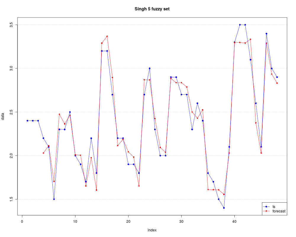
> #Sing model
> fuzzy.ts1(lh,n=5,type="Singh",plot=TRUE)
Time Series:
Start = 1 
End = 48 
Frequency = 1 
 [1]       NA       NA       NA 2.030000 2.113333 1.705000 2.475000 2.364286
 [9] 2.461111 2.010000 2.004286 1.652500 1.976667 1.605000 3.290000 3.368889
[17] 2.895556 2.115000 2.186923 2.042917 1.982857 1.653333 2.870000 2.867778
[25] 2.425000 2.092667 2.038333 2.885000 2.836250 2.836250 2.786667 2.500000
[33] 2.429167 2.525000 1.610000 1.608667 1.607000 1.555455 2.030000 3.295000
[41] 3.298000 3.291111 3.334444 2.375000 2.030000 3.290000 2.935000 2.831667
> 
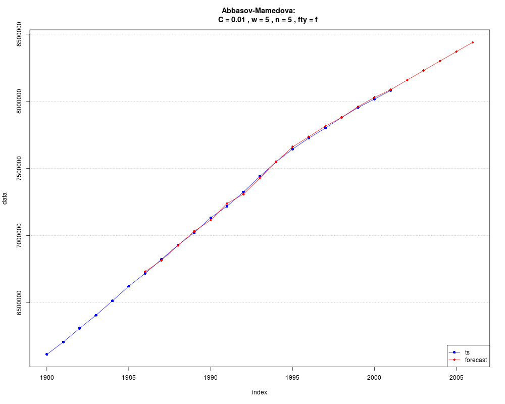
> #Abbasov Mamedova model
> data(population)
> fuzzy.ts2(population,n=5,w=5,C=0.01,forecast=5,fty="f",plot=TRUE)
$timeseries
Time Series:
Start = 1986 
End = 2006 
Frequency = 1 
 [1] 6730413 6815006 6925418 7031666 7114728 7238471 7307996 7428376 7547883
[10] 7659971 7736224 7815092 7879486 7959942 8029016 8087173 8158406 8229322
[19] 8299869 8369905 8439408

$accuracy
                        ME     MAE    MPE  MAPE       MSE     RMSE     U
Abbasov.Mamedova -3322.622 10460.9 -0.042 0.142 142118608 11921.35 0.129

> 
> #Improve Abbasov Mamedova version 1 model
> data(sanility)
> fuzzy.ts3(sanility,n=5,w=5,C=0.01,forecast=5,fty="ts")
$timeseries
Time Series:
Start = 2005 
End = 2020 
Frequency = 1 
 [1] 36.15852 31.63274 32.95609 31.54294 28.33426 37.18810 28.40924 27.34420
 [9] 33.17655 31.34119 33.15838 33.20842 33.25842 33.30842 33.35842 33.40842

$accuracy
          ME          MAE          MPE         MAPE          MSE         RMSE 
-0.049291435  0.049291435 -0.151336880  0.151336880  0.002856891  0.053449896 

> 
> 
> 
> 
> 
> dev.off()
null device 
          1 
>