Supported by Dr. Osamu Ogasawara and  . . |
|
Last data update: 2014.03.03 |
DescriptivesDescriptionThis function calculate to return answer which are descriptive statistics values for a continuously variable or continuously variables in data frame. UsageDescriptives(x, plot = FALSE, r = 2, answer = 1, statistic = "ALL") Arguments
DetailsStatistic descriptive values are calculated by theory of base statistic. Value
NoteYou must not withdraw discrete variables from data frame. When you let a data frame in to this function which will auto withdraw discrete variables and calculate descriptive statistic to continuously variables. Author(s)Mai Thi Hong Diem <maidiemks@gmail.com> Hong Viet Minh <hongvietminh@gmail.com> ReferencesTheory of base statistic. See Also
Examples
#Load data
library(MASS)
data(crabs)
#Calculate descriptive statistic to a continuously variable
Descriptives(crabs$FL)
#Calculate descriptive statistic to continuously variables
Descriptives(crabs)
Descriptives(crabs,answer=2)
Descriptives(crabs,answer=2,r=6)
#To just see some descriptive statistic variables
Descriptives(crabs,statistic=list("Min","Mean","Median","Max"))
#Combined paint graph to compare
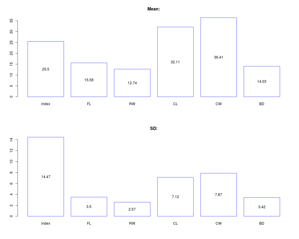
Descriptives(crabs,plot=list("Mean","SD"))
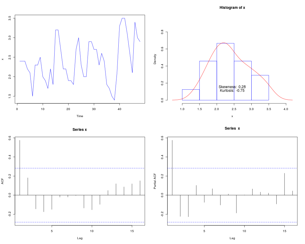
#Descriptives for time series
Descriptives(lh,plot=TRUE)
Results
R version 3.3.1 (2016-06-21) -- "Bug in Your Hair"
Copyright (C) 2016 The R Foundation for Statistical Computing
Platform: x86_64-pc-linux-gnu (64-bit)

R is free software and comes with ABSOLUTELY NO WARRANTY.
You are welcome to redistribute it under certain conditions.
Type 'license()' or 'licence()' for distribution details.

R is a collaborative project with many contributors.
Type 'contributors()' for more information and
'citation()' on how to cite R or R packages in publications.

Type 'demo()' for some demos, 'help()' for on-line help, or
'help.start()' for an HTML browser interface to help.
Type 'q()' to quit R.

> library(AnalyzeTS)
Loading required package: MASS
Loading required package: TSA
Loading required package: leaps
Loading required package: locfit
locfit 1.5-9.1 	 2013-03-22
Loading required package: mgcv
Loading required package: nlme
This is mgcv 1.8-12. For overview type 'help("mgcv-package")'.
Loading required package: tseries

Attaching package: 'TSA'

The following objects are masked from 'package:stats':

    acf, arima

The following object is masked from 'package:utils':

    tar

Loading required package: TTR
> png(filename="/home/ddbj/snapshot/RGM3/R_CC/result/AnalyzeTS/Descriptives.Rd_%03d_medium.png", width=480, height=480)
> ### Name: Descriptives
> ### Title: Descriptives
> ### Aliases: Descriptives
> ### Keywords: Descriptives
>
> ### ** Examples
>
> #Load data
> library(MASS)
> data(crabs)
>
> #Calculate descriptive statistic to a continuously variable
> Descriptives(crabs$FL)
             x
N:      200.00
NaN:      0.00
Min:      7.20
1sq QU:  12.90
Median:  15.55
Mean:    15.58
3rd QU:  18.05
Max:     23.10
VAR:     12.22
SD:       3.50
SE:       0.25
>
> #Calculate descriptive statistic to continuously variables
> Descriptives(crabs)
         index     FL     RW     CL     CW     BD
N:      200.00 200.00 200.00 200.00 200.00 200.00
NaN:      0.00   0.00   0.00   0.00   0.00   0.00
Min:      1.00   7.20   6.50  14.70  17.10   6.10
1sq QU:  13.00  12.90  11.00  27.28  31.50  11.40
Median:  25.50  15.55  12.80  32.10  36.80  13.90
Mean:    25.50  15.58  12.74  32.11  36.41  14.03
3rd QU:  38.00  18.05  14.30  37.23  42.00  16.60
Max:     50.00  23.10  20.20  47.60  54.60  21.60
VAR:    209.30  12.22   6.62  50.68  61.97  11.73
SD:      14.47   3.50   2.57   7.12   7.87   3.42
SE:       1.02   0.25   0.18   0.50   0.56   0.24
> Descriptives(crabs,answer=2)
       N: NaN: Min: 1sq QU: Median: Mean: 3rd QU: Max:   VAR:   SD:  SE:
index 200    0  1.0   13.00   25.50 25.50   38.00 50.0 209.30 14.47 1.02
FL    200    0  7.2   12.90   15.55 15.58   18.05 23.1  12.22  3.50 0.25
RW    200    0  6.5   11.00   12.80 12.74   14.30 20.2   6.62  2.57 0.18
CL    200    0 14.7   27.28   32.10 32.11   37.23 47.6  50.68  7.12 0.50
CW    200    0 17.1   31.50   36.80 36.41   42.00 54.6  61.97  7.87 0.56
BD    200    0  6.1   11.40   13.90 14.03   16.60 21.6  11.73  3.42 0.24
> Descriptives(crabs,answer=2,r=6)
       N: NaN: Min: 1sq QU: Median:   Mean: 3rd QU: Max:       VAR:       SD:
index 200    0  1.0  13.000   25.50 25.5000  38.000 50.0 209.296482 14.467083
FL    200    0  7.2  12.900   15.55 15.5830  18.050 23.1  12.217297  3.495325
RW    200    0  6.5  11.000   12.80 12.7385  14.300 20.2   6.622078  2.573340
CL    200    0 14.7  27.275   32.10 32.1055  37.225 47.6  50.679919  7.118983
CW    200    0 17.1  31.500   36.80 36.4145  42.000 54.6  61.967678  7.871955
BD    200    0  6.1  11.400   13.90 14.0305  16.600 21.6  11.729065  3.424772
           SE:
index 1.022977
FL    0.247157
RW    0.181963
CL    0.503388
CW    0.556631
BD    0.242168
>
> #To just see some descriptive statistic variables
> Descriptives(crabs,statistic=list("Min","Mean","Median","Max"))
        index    FL    RW    CL    CW    BD
Min:      1.0  7.20  6.50 14.70 17.10  6.10
Median:  25.5 15.55 12.80 32.10 36.80 13.90
Mean:    25.5 15.58 12.74 32.11 36.41 14.03
Max:     50.0 23.10 20.20 47.60 54.60 21.60
>
> #Combined paint graph to compare
> Descriptives(crabs,plot=list("Mean","SD"))
         index     FL     RW     CL     CW     BD
N:      200.00 200.00 200.00 200.00 200.00 200.00
NaN:      0.00   0.00   0.00   0.00   0.00   0.00
Min:      1.00   7.20   6.50  14.70  17.10   6.10
1sq QU:  13.00  12.90  11.00  27.28  31.50  11.40
Median:  25.50  15.55  12.80  32.10  36.80  13.90
Mean:    25.50  15.58  12.74  32.11  36.41  14.03
3rd QU:  38.00  18.05  14.30  37.23  42.00  16.60
Max:     50.00  23.10  20.20  47.60  54.60  21.60
VAR:    209.30  12.22   6.62  50.68  61.97  11.73
SD:      14.47   3.50   2.57   7.12   7.87   3.42
SE:       1.02   0.25   0.18   0.50   0.56   0.24
>
> #Descriptives for time series
> Descriptives(lh,plot=TRUE)
            x
N:      48.00
NaN:     0.00
Min:     1.40
1sq QU:  2.00
Median:  2.30
Mean:    2.40
3rd QU:  2.75
Max:     3.50
VAR:     0.30
SD:      0.55
SE:      0.08
>
>
>
>
>
> dev.off()
null device
          1
>
|