R Graphical Manual

Browse All

Last data update: 2014.03.03

R: Abbasov Mamedova model

fuzzy.ts2

R Documentation

Abbasov Mamedova model

Description

Predicts time series by fuzziness method according to Abbasov-Manedova model.

Usage

fuzzy.ts2(ts, n = 5, w = NULL, D1 = 0, D2 = 0, C = NULL, trace = FALSE,
forecast = NULL, plot = FALSE, fty = c("ts", "f"))

Arguments

`ts`	Observation series.
`n`	Number of fuzzy set.
`w`	The 'w' parameter.
`D1`	A adequate value.
`D2`	A adequate value.
`C`	A optional constant.
`trace`	Let trace=TRUE to print all of calculation results out to creen. Let trace=FALSE (default) to only print forecasting series out to creen.
`forecast`	Number of points to forecast in future.
`plot`	Let plot=TRUE to paint graph of obsevation series and fuzzy series. Let plot=FLASE (default) to do not paint graph.
`fty`	fty="f", N(length(ts)+1) = N(length(ts)) + V(length(ts)+1). fty="ts", N(length(ts)+1) = ts(length(ts)) + V(length(ts)+1).

Value

`type`	Name of fuzzy model.
`table1`	Information about changing fuzzy sets.
`table2`	Observation series and changing series.
`table3`	The change fuzzy of observation series.
`table4`	Interpolate values.
`table5`	Forecasting values.
`table6`	The change fuzzy of forecasting series.
`timeseries`	Forecasting timeseries.
`accuracy`	Information about 7 accuracy of forecasting model.

Author(s)

Doan Hai Nghi <Hainghi1426262609121094@gmail.com>

Tran Thi Ngoc Han <tranthingochan01011994@gmail.com>

Hong Viet Minh <hongvietminh@gmail.com>

References

Abbasov, A.M. and Mamedova, M.H., 2003. Application of fuzzy time series to population forecasting, Proceedings of 8th Symposion on Information Technology in Urban and Spatial Planning, Vienna University of Technology, February 25-March1, 545-552.

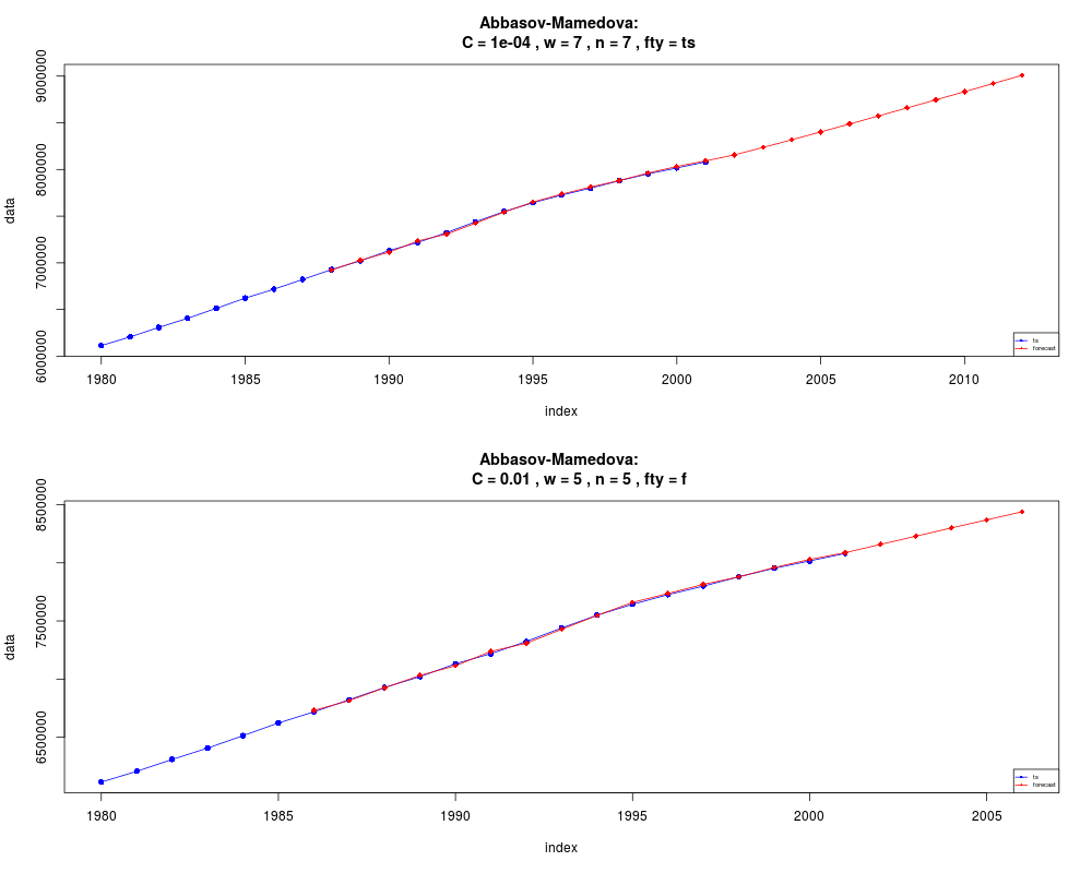
Examples

data(population)
layout(1:2)
fuzzy.ts2(population,n=7,w=7,C=0.0001,forecast=11,fty="ts",trace=TRUE,plot=TRUE)
fuzzy.ts2(population,n=5,w=5,C=0.01,forecast=5,fty="f",plot=TRUE)

Results


R version 3.3.1 (2016-06-21) -- "Bug in Your Hair"
Copyright (C) 2016 The R Foundation for Statistical Computing
Platform: x86_64-pc-linux-gnu (64-bit)

R is free software and comes with ABSOLUTELY NO WARRANTY.
You are welcome to redistribute it under certain conditions.
Type 'license()' or 'licence()' for distribution details.

R is a collaborative project with many contributors.
Type 'contributors()' for more information and
'citation()' on how to cite R or R packages in publications.

Type 'demo()' for some demos, 'help()' for on-line help, or
'help.start()' for an HTML browser interface to help.
Type 'q()' to quit R.

> library(AnalyzeTS)
Loading required package: MASS
Loading required package: TSA
Loading required package: leaps
Loading required package: locfit
locfit 1.5-9.1 	 2013-03-22
Loading required package: mgcv
Loading required package: nlme
This is mgcv 1.8-12. For overview type 'help("mgcv-package")'.
Loading required package: tseries

Attaching package: 'TSA'

The following objects are masked from 'package:stats':

    acf, arima

The following object is masked from 'package:utils':

    tar

Loading required package: TTR
> png(filename="/home/ddbj/snapshot/RGM3/R_CC/result/AnalyzeTS/fuzzy.ts2.Rd_%03d_medium.png", width=480, height=480)
> ### Name: fuzzy.ts2
> ### Title: Abbasov Mamedova model
> ### Aliases: fuzzy.ts2
> ### Keywords: fuzzy.ts2
> 
> ### ** Examples
> 
> data(population)
> layout(1:2)
> fuzzy.ts2(population,n=7,w=7,C=0.0001,forecast=11,fty="ts",trace=TRUE,plot=TRUE)
$type
[1] "Abbasov-Manedova"

$table1
   U       low        up        Bw
1 u1  62800.00  70385.71  66592.86
2 u2  70385.71  77971.43  74178.57
3 u3  77971.43  85557.14  81764.29
4 u4  85557.14  93142.86  89350.00
5 u5  93142.86 100728.57  96935.71
6 u6 100728.57 108314.29 104521.43
7 u7 108314.29 115900.00 112107.14

$table2
   point      ts diff.ts
1   1980 6114300      NA
2   1981 6206700   92400
3   1982 6308800  102100
4   1983 6406300   97500
5   1984 6513300  107000
6   1985 6622400  109100
7   1986 6717900   95500
8   1987 6822700  104800
9   1988 6928000  105300
10  1989 7021200   93200
11  1990 7131900  110700
12  1991 7218500   86600
13  1992 7324100  105600
14  1993 7440000  115900
15  1994 7549600  109600
16  1995 7643500   93900
17  1996 7726200   82700
18  1997 7799800   73600
19  1998 7879700   79900
20  1999 7953400   73700
21  2000 8016200   62800
22  2001 8081000   64800

$table3
 [1] NA                                                                                                                                                                             
 [2] "A[1981]={(0.130546833376749/u1),(0.231470519217899/u2),(0.469222701473096/u3),(0.914892157086983/u4),(0.829375112399369/u5),(0.404974659123945/u6),(0.204762161958304/u7)}"   
 [3] "A[1982]={(0.0734884962945113/u1),(0.113687242104696/u2),(0.194726314648515/u3),(0.380861699595334/u4),(0.789453863067617/u5),(0.944614276880903/u6),(0.499642984693845/u7)}"  
 [4] "A[1983]={(0.0947641409976314/u1),(0.155306264349487/u2),(0.287676482550293/u3),(0.6008802896243/u4),(0.996825923170151/u5),(0.669790304375269/u6),(0.319112996120986/u7)}"    
 [5] "A[1984]={(0.0577121564385758/u1),(0.084944000884111/u2),(0.135714438541405/u3),(0.243000078975026/u4),(0.49679604570625/u5),(0.942122438424367/u6),(0.793128913797813/u7)}"   
 [6] "A[1985]={(0.052442312052038/u1),(0.0757859281075352/u2),(0.11803013249063/u3),(0.204055605152404/u4),(0.403274838592332/u5),(0.826696911401289/u6),(0.917070185346435/u7)}"   
 [7] "A[1986]={(0.106880666481661/u1),(0.180309055240347/u2),(0.346416506817247/u3),(0.725570933628399/u4),(0.979803549388347/u5),(0.551309937727293/u6),(0.266100975816716/u7)}"   
 [8] "A[1987]={(0.0641113685124406/u1),(0.0963695761444784/u2),(0.158568033574354/u3),(0.295244351606498/u4),(0.617867531092765/u5),(0.999224581332548/u6),(0.651914549967754/u7)}" 
 [9] "A[1988]={(0.0625687118580255/u1),(0.0935853497673663/u2),(0.152921602321912/u3),(0.282165052447429/u4),(0.588369319421801/u5),(0.993974788539471/u6),(0.68335327028121/u7)}"  
[10] "A[1989]={(0.123771559379563/u1),(0.216537044572051/u2),(0.433321446471205/u3),(0.870909447190228/u4),(0.877535057749418/u5),(0.438260597353666/u6),(0.218588766388721/u7)}"   
[11] "A[1990]={(0.048889235326214/u1),(0.0697440170397444/u2),(0.106692208926643/u3),(0.179913551538486/u4),(0.345476174570521/u5),(0.723721256542569/u6),(0.980583937734921/u7)}"  
[12] "A[1991]={(0.199885759169683/u1),(0.393248879792444/u2),(0.810476986381919/u3),(0.929692039511912/u4),(0.483495892381708/u5),(0.23742952976476/u6),(0.133224207300673/u7)}"    
[13] "A[1992]={(0.0616691168079461/u1),(0.0919704149944435/u2),(0.149668945274543/u3),(0.274678111587983/u4),(0.571200590784611/u5),(0.988500611004332/u6),(0.702528852967521/u7)}" 
[14] "A[1993]={(0.0395070416161734/u1),(0.054327819216753/u2),(0.0790359517204856/u3),(0.124238650022829/u4),(0.217559613831686/u5),(0.435783228082049/u6),(0.874234654394077/u7)}" 
[15] "A[1994]={(0.0512921956490558/u1),(0.0738183017489551/u2),(0.114308316005806/u3),(0.196054405097415/u4),(0.384047979349192/u5),(0.794963823062143/u6),(0.940859763412172/u7)}" 
[16] "A[1995]={(0.118248029948606/u1),(0.204526270721198/u2),(0.404407129862764/u3),(0.828483254282223/u4),(0.915620437956204/u5),(0.469892253226853/u6),(0.231749682910861/u7)}"   
[17] "A[1996]={(0.27821051025369/u1),(0.579324785139964/u2),(0.991320383114981/u3),(0.693373086723639/u4),(0.330408599119798/u5),(0.173558457543484/u6),(0.103650567706322/u7)}"    
[18] "A[1997]={(0.670690582032815/u1),(0.996663719050668/u2),(0.600039982255961/u3),(0.287304722571377/u4),(0.155145663176074/u5),(0.0946848879682126/u6),(0.0631791741070083/u7)}" 
[19] "A[1998]={(0.360906530916708/u1),(0.753382244241142/u2),(0.966411767345242/u3),(0.528255041534053/u4),(0.256268611344462/u5),(0.141599988845389/u6),(0.0879275437561776/u7)}"  
[20] "A[1999]={(0.664401149142804/u1),(0.997714927393332/u2),(0.605940504680427/u3),(0.289920199465097/u4),(0.15627480414023/u5),(0.0952416818417603/u6),(0.063487684960114/u7)}"   
[21] "A[2000]={(0.874234654394077/u1),(0.435783228082049/u2),(0.217559613831686/u3),(0.124238650022829/u4),(0.0790359517204856/u5),(0.0543278192167531/u6),(0.0395070416161734/u7)}"
[22] "A[2001]={(0.968857652566657/u1),(0.532034878686547/u2),(0.257873530137324/u3),(0.142307733358/u4),(0.0882843075409077/u5),(0.0596021477573126/u6),(0.0427722259598213/u7)}"   

$table4
   point interpolate diff.interpolate
1   1988     6922560         99860.14
2   1989     7028233        100232.51
3   1990     7114173         92973.41
4   1991     7234418        102517.61
5   1992     7308215         89715.27
6   1993     7424500        100399.65
7   1994     7543508        103508.07
8   1995     7651955        102354.50
9   1996     7736103         92603.10
10  1997     7812161         85961.44
11  1998     7881559         81759.20
12  1999     7962303         82602.84
13  2000     8032039         78638.75
14  2001     8092472         76271.60

$table5
   point forecast diff.forecast
1   2002  8156642      75642.37
2   2003  8236437      79794.77
3   2004  8318968      82531.03
4   2005  8402497      83528.58
5   2006  8487269      84772.16
6   2007  8572845      85576.58
7   2008  8659166      86320.36
8   2009  8746052      86885.85
9   2010  8833414      87362.41
10  2011  8921155      87741.17
11  2012  9009206      88050.95

$table6
 [1] "A[2002]={(0.549771876254875/u1),(0.979022513653749/u2),(0.727389688385735/u3),(0.347343784578306/u4),(0.180698950565954/u5),(0.107066357544661/u6),(0.0699457275337394/u7)}"
 [2] "A[2003]={(0.364577130869072/u1),(0.760215581388462/u2),(0.962658381129771/u3),(0.522732297322075/u4),(0.25392818652942/u5),(0.140566338570753/u6),(0.0874057310023975/u7)}" 
 [3] "A[2004]={(0.28246558344442/u1),(0.589054410060232/u2),(0.994155355533527/u3),(0.682601689992537/u4),(0.325208688516476/u5),(0.171356839671047/u6),(0.102590796333564/u7)}"  
 [4] "A[2005]={(0.258519078666775/u1),(0.533553511014876/u2),(0.969812380375244/u3),(0.746887612885214/u4),(0.357460359421135/u5),(0.184945520198257/u6),(0.109082853546951/u7)}" 
 [5] "A[2006]={(0.232294971784355/u1),(0.471199853143914/u2),(0.917033052131337/u3),(0.826742850224504/u4),(0.403303883831953/u5),(0.204067679111724/u6),(0.118035723611513/u7)}" 
 [6] "A[2007]={(0.217211097667399/u1),(0.434944219863876/u2),(0.873106479007171/u3),(0.87535996073922/u4),(0.436624039348436/u5),(0.217908891487582/u6),(0.124398083541304/u7)}"  
 [7] "A[2008]={(0.204426152712379/u1),(0.404166264554157/u2),(0.828104034422575/u3),(0.915929200999427/u4),(0.470177053223571/u5),(0.231868437836358/u6),(0.130726064864348/u7)}" 
 [8] "A[2009]={(0.195386698275761/u1),(0.382445837082818/u2),(0.792202051873913/u3),(0.942755559992384/u4),(0.497513012095662/u5),(0.243300937262848/u6),(0.13584859674632/u7)}"  
 [9] "A[2010]={(0.18819119591747/u1),(0.365211819547439/u2),(0.761388243811042/u3),(0.961996346956103/u4),(0.521789727305642/u5),(0.253529262942909/u6),(0.140389966998187/u7)}"  
[10] "A[2011]={(0.182731471882317/u1),(0.352182045988528/u2),(0.736794051824352/u3),(0.974769682072755/u4),(0.541888941300523/u5),(0.262070232601754/u6),(0.144154394595094/u7)}" 
[11] "A[2012]={(0.178428093676838/u1),(0.341947026218171/u2),(0.716731919594992/u3),(0.98340480564729/u4),(0.5588496927048/u5),(0.269340985819458/u6),(0.147340440692504/u7)}"    

$accuracy
                        ME      MAE    MPE  MAPE       MSE     RMSE     U
Abbasov.Mamedova -2221.293 10884.65 -0.026 0.145 140277411 11843.88 0.129

> fuzzy.ts2(population,n=5,w=5,C=0.01,forecast=5,fty="f",plot=TRUE)
$timeseries
Time Series:
Start = 1986 
End = 2006 
Frequency = 1 
 [1] 6730413 6815006 6925418 7031666 7114728 7238471 7307996 7428376 7547883
[10] 7659971 7736224 7815092 7879486 7959942 8029016 8087173 8158406 8229322
[19] 8299869 8369905 8439408

$accuracy
                        ME     MAE    MPE  MAPE       MSE     RMSE     U
Abbasov.Mamedova -3322.622 10460.9 -0.042 0.142 142118608 11921.35 0.129

> 
> 
> 
> 
> 
> dev.off()
null device 
          1 
>