Improve Abbasov Mamedova version 1 model

Description

Predicts time series by fuzziness method according to improve Abbasov-Manedova model.

Usage

fuzzy.ts3(ts, n = 7, w = 7, D1 = 0, D2 = 0, C = NULL, forecast = 5, 
fty = c("ts", "f"), trace = FALSE, plot = FALSE)

Arguments

Value

Author(s)

Hong Viet Minh <hongvietminh@gmail.com>

Vo Van Tai <vvtai@ctu.edu.vn>

References

Vo Van Tai, Duong Ton Dam, Pham Minh Truc, Dang Kien Cuong, 2016. Forecasting crest of sanility at three main stations of Ca Mau province by fuzzy time series model.

See Also

fuzzy.ts2

Examples

data(sanility)
fuzzy.ts3(sanility,n=7,w=4,C=0.01,forecast=5,fty="f",plot=TRUE,trace=1)
fuzzy.ts3(sanility,n=5,w=5,C=0.01,forecast=5,fty="ts")

Results

R version 3.3.1 (2016-06-21) -- "Bug in Your Hair"
Copyright (C) 2016 The R Foundation for Statistical Computing
Platform: x86_64-pc-linux-gnu (64-bit)

R is free software and comes with ABSOLUTELY NO WARRANTY.
You are welcome to redistribute it under certain conditions.
Type 'license()' or 'licence()' for distribution details.

R is a collaborative project with many contributors.
Type 'contributors()' for more information and
'citation()' on how to cite R or R packages in publications.

Type 'demo()' for some demos, 'help()' for on-line help, or
'help.start()' for an HTML browser interface to help.
Type 'q()' to quit R.

> library(AnalyzeTS)
Loading required package: MASS
Loading required package: TSA
Loading required package: leaps
Loading required package: locfit
locfit 1.5-9.1 	 2013-03-22
Loading required package: mgcv
Loading required package: nlme
This is mgcv 1.8-12. For overview type 'help("mgcv-package")'.
Loading required package: tseries

Attaching package: 'TSA'

The following objects are masked from 'package:stats':

    acf, arima

The following object is masked from 'package:utils':

    tar

Loading required package: TTR
> png(filename="/home/ddbj/snapshot/RGM3/R_CC/result/AnalyzeTS/fuzzy.ts3.Rd_%03d_medium.png", width=480, height=480)
> ### Name: fuzzy.ts3
> ### Title: Improve Abbasov Mamedova version 1 model
> ### Aliases: fuzzy.ts3
> ### Keywords: fuzzy.ts3
> 
> ### ** Examples
> 
> data(sanility)
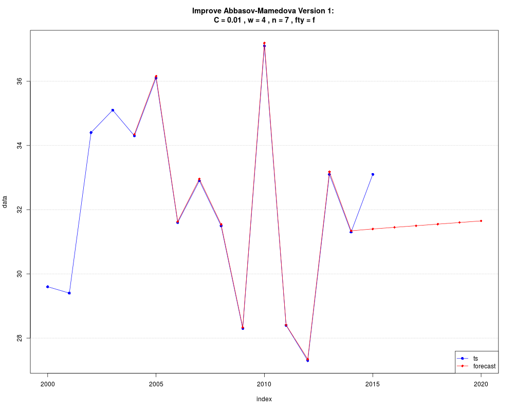
> fuzzy.ts3(sanility,n=7,w=4,C=0.01,forecast=5,fty="f",plot=TRUE,trace=1)
$type
[1] "Improve Abbasov-Manedova"

$table1
   U  low   up    Bw
1 u1 -8.7 -6.2 -7.45
2 u2 -6.2 -3.7 -4.95
3 u3 -3.7 -1.2 -2.45
4 u4 -1.2  1.3  0.05
5 u5  1.3  3.8  2.55
6 u6  3.8  6.3  5.05
7 u7  6.3  8.8  7.55

$table2
   point   ts diff.ts
1   2000 29.6      NA
2   2001 29.4    -0.2
3   2002 34.4     5.0
4   2003 35.1     0.7
5   2004 34.3    -0.8
6   2005 36.1     1.8
7   2006 31.6    -4.5
8   2007 32.9     1.3
9   2008 31.5    -1.4
10  2009 28.3    -3.2
11  2010 37.1     8.8
12  2011 28.4    -8.7
13  2012 27.3    -1.1
14  2013 33.1     5.8
15  2014 31.3    -1.8
16  2015 33.1     1.8

$table3
 [1] NA                                                                                                                                                                          
 [2] "A[2001]={(0.994771233702849/u1),(0.997748829204108/u2),(0.999494006159382/u3),(0.999993750039062/u4),(0.999244321481879/u5),(0.997251326032623/u6),(0.994029609656998/u7)}"
 [3] "A[2002]={(0.984736340537582/u1),(0.990196804090305/u2),(0.994480385241812/u3),(0.997555739050392/u4),(0.999400110083922/u5),(0.999999750000062/u6),(0.999350172550299/u7)}"
 [4] "A[2003]={(0.993401578366098/u1),(0.996817908033081/u2),(0.999008733584101/u3),(0.999957751784987/u4),(0.999657867094987/u5),(0.99811132384745/u6),(0.995329664382302/u7)}" 
 [5] "A[2004]={(0.995597220193002/u1),(0.998280711045402/u2),(0.999727824099889/u3),(0.999927755219685/u4),(0.998879008033235/u5),(0.99658942185107/u6),(0.993076025679953/u7)}" 
 [6] "A[2005]={(0.991516338330163/u1),(0.995464415257981/u2),(0.998197006656726/u3),(0.999693843760348/u4),(0.999943753163884/u5),(0.998944864486886/u6),(0.996704645266587/u7)}"
 [7] "A[2006]={(0.999130506676565/u1),(0.999979750410054/u2),(0.999579926535873/u3),(0.997934027080437/u4),(0.995054331210302/u5),(0.990962177203361/u6),(0.985687570060824/u7)}"
 [8] "A[2007]={(0.992401922778725/u1),(0.996108949416342/u2),(0.998595724762053/u3),(0.999843774410248/u4),(0.999843774410248/u5),(0.998595724762053/u6),(0.996108949416342/u7)}"
 [9] "A[2008]={(0.996353098570956/u1),(0.998741336231015/u2),(0.999889762153722/u3),(0.99978979419577/u4),(0.998442180587738/u5),(0.995856985974101/u6),(0.992053404218856/u7)}" 
[10] "A[2009]={(0.998197006656726/u1),(0.999693843760348/u2),(0.999943753163884/u3),(0.998944864486886/u4),(0.996704645266587/u5),(0.993239761870767/u6),(0.988575771243567/u7)}"
[11] "A[2010]={(0.974273100928604/u1),(0.981444563717221/u2),(0.987501928714704/u3),(0.992401922778725/u4),(0.996108949416342/u5),(0.998595724762053/u6),(0.999843774410248/u7)}"
[12] "A[2011]={(0.999843774410248/u1),(0.998595724762053/u2),(0.996108949416342/u3),(0.992401922778725/u4),(0.987501928714704/u5),(0.981444563717221/u6),(0.974273100928604/u7)}"
[13] "A[2012]={(0.995983943742843/u1),(0.998519943813283/u2),(0.99981778320901/u3),(0.99986776748775/u4),(0.998669522528611/u5),(0.99623200151228/u6),(0.99257331828923/u7)}"    
[14] "A[2013]={(0.982746654054751/u1),(0.988575771243567/u2),(0.993239761870767/u3),(0.996704645266587/u4),(0.998944864486886/u5),(0.999943753163884/u6),(0.999693843760348/u7)}"
[15] "A[2014]={(0.996817908033081/u1),(0.999008733584101/u2),(0.999957751784987/u3),(0.999657867094987/u4),(0.99811132384745/u5),(0.995329664382302/u6),(0.991333514582144/u7)}" 
[16] "A[2015]={(0.991516338330163/u1),(0.995464415257981/u2),(0.998197006656726/u3),(0.999693843760348/u4),(0.999943753163884/u5),(0.998944864486886/u6),(0.996704645266587/u7)}"

$table4
   point interpolate diff.interpolate
5   2004    34.34713               NA
6   2005    36.15859      0.047127909
7   2006    31.63245      0.058590997
8   2007    32.95621      0.032446166
9   2008    31.54291      0.056210228
10  2009    28.33389      0.042907159
11  2010    37.18913      0.033886952
12  2011    28.40862      0.089131561
13  2012    27.34358      0.008619948
14  2013    33.17742      0.043580215
15  2014    31.34116      0.077417634
16  2015    31.39949      0.041155820

$table5
  point forecast diff.forecast
1  2016 31.44953    0.05833648
2  2017 31.49953    0.05004143
3  2018 31.54953    0.05000021
4  2019 31.59953    0.05000010
5  2020 31.64953    0.05000000
6  2021       NA    0.05000000

$table6
[1] "A[2016]={(0.994394091700727/u1),(0.997497932612568/u2),(0.9993712204218/u3),(0.999999993050307/u4),(0.999379546492879/u5),(0.997514522523169/u6),(0.99441882214649/u7)}"   
[2] "A[2017]={(0.994406402197001/u1),(0.997506193194785/u2),(0.999375369694026/u3),(0.999999999999828/u4),(0.999375411067656/u5),(0.997506275632807/u6),(0.994406525086695/u7)}"
[3] "A[2018]={(0.994406463336697/u1),(0.99750623420915/u2),(0.99937539027822/u3),(1/u4),(0.999375390483804/u5),(0.99750623461878/u6),(0.99440646394733/u7)}"                    
[4] "A[2019]={(0.994406463488596/u1),(0.997506234311048/u2),(0.99937539032936/u3),(1/u4),(0.999375390432663/u5),(0.997506234516882/u6),(0.994406463795431/u7)}"                 
[5] "A[2020]={(0.994406463640874/u1),(0.997506234413201/u2),(0.999375390380628/u3),(1/u4),(0.999375390381396/u5),(0.99750623441473/u6),(0.994406463643153/u7)}"                 
[6] "A[2021]={(0.99440646364163/u1),(0.997506234413708/u2),(0.999375390380883/u3),(1/u4),(0.999375390381141/u5),(0.997506234414223/u6),(0.994406463642398/u7)}"                 

$accuracy
        ME        MAE        MPE       MAPE        MSE       RMSE 
0.09745276 0.18596519 0.29272402 0.56352356 0.24351561 0.49347301 

> fuzzy.ts3(sanility,n=5,w=5,C=0.01,forecast=5,fty="ts")
$timeseries
Time Series:
Start = 2005 
End = 2020 
Frequency = 1 
 [1] 36.15852 31.63274 32.95609 31.54294 28.33426 37.18810 28.40924 27.34420
 [9] 33.17655 31.34119 33.15838 33.20842 33.25842 33.30842 33.35842 33.40842

$accuracy
          ME          MAE          MPE         MAPE          MSE         RMSE 
-0.049291435  0.049291435 -0.151336880  0.151336880  0.002856891  0.053449896 

> 
> 
> 
> 
> 
> dev.off()
null device 
          1 
>