R Graphical Manual

Browse All

Last data update: 2014.03.03

R: Archetypal analysis in multivariate accommodation problem

archetypesBoundary

R Documentation

Archetypal analysis in multivariate accommodation problem

Description

This function allows us to reproduce the results shown in section 2.2.2 and section 3.1 of Epifanio et al. (2013). In addition, from the results provided by this function, the other results shown in section 3.2 and section 3.3 of the same paper can be also reproduced (see section examples below).

Usage

archetypesBoundary(data,numArch,verbose,numRep)

Arguments

`data`	USAF 1967 database (see `USAFSurvey`). Each row corresponds to an observation, and each column corresponds to a variable. All variables are numeric.
`numArch`	Number of archetypes (archetypal observations).
`verbose`	Logical value. If TRUE, some details of the execution progress are shown (this is the same argument as that of the `stepArchetypes` function of the archetypes R package (Eugster (2009))).
`numRep`	For each archetype run `archetypes` `numRep` times (this is the same argument as the `nrep` argument of the `stepArchetypes` function of archetypes).

Details

Before using this function, the more extreme (100 - percAcomm*100)% observations must be removed by means of the preprocessing function. To that end, it is recommended that you use the Mahalanobis distance. In this case, the depth procedure has the disadvantage that the desired percentage of accommodation is not under control of the analyst and it may not exactly coincide with that one indicated.

Value

A list with numArch elements. Each element is a list of class attribute stepArchetypes with numRep elements.

Note

We would like to note that, some time after publishing the paper Epifanio et al. (2013), we found out that the stepArchetypes function standardizes the data by default (even when the data are already standardized) and this option is not always desired. In order to avoid this way of proceeding, we have created the stepArchetypesRawData function, which is used within archetypesBoundary instead of using stepArchetypes. Therefore, the results provided by archetypesBoundary allows us to reproduce the results of Epifanio et al. (2013) but they are now slightly different.

Author(s)

Irene Epifanio and Guillermo Vinue

References

Epifanio, I., Vinue, G., and Alemany, S., (2013). Archetypal analysis: contributions for estimating boundary cases in multivariate accommodation problem, Computers & Industrial Engineering 64, 757–765.

Eugster, M. J., and Leisch, F., (2009). From Spider-Man to Hero - Archetypal Analysis in R, Journal of Statistical Software 30, 1–23, http://www.jstatsoft.org/.

Zehner, G. F., Meindl, R. S., and Hudson, J. A., (1993). A multivariate anthropometric method for crew station design: abridged. Tech. rep. Ohio: Human Engineering Division, Armstrong Laboratory, Wright-Patterson Air Force Base.

Examples

#The following R code allows us to reproduce the results of the paper Epifanio et al. (2013).
#As a toy example, only the first 25 individuals are used.
#First,the USAF 1967 database is read and preprocessed (Zehner et al. (1993)).
#Variable selection:
variabl_sel <- c(48, 40, 39, 33, 34, 36)
#Changing to inches: 
USAFSurvey_inch <- USAFSurvey[1:25, variabl_sel] / (10 * 2.54)

#Data preprocessing:
USAFSurvey_preproc <- preprocessing(USAFSurvey_inch, TRUE, 0.95, TRUE)

#Procedure and results shown in section 2.2.2 and section 3.1:
set.seed(2010)
res <- archetypesBoundary(USAFSurvey_preproc$data, 15, FALSE, 3)
#To understand the warning messages, see the vignette of the
#archetypes package.

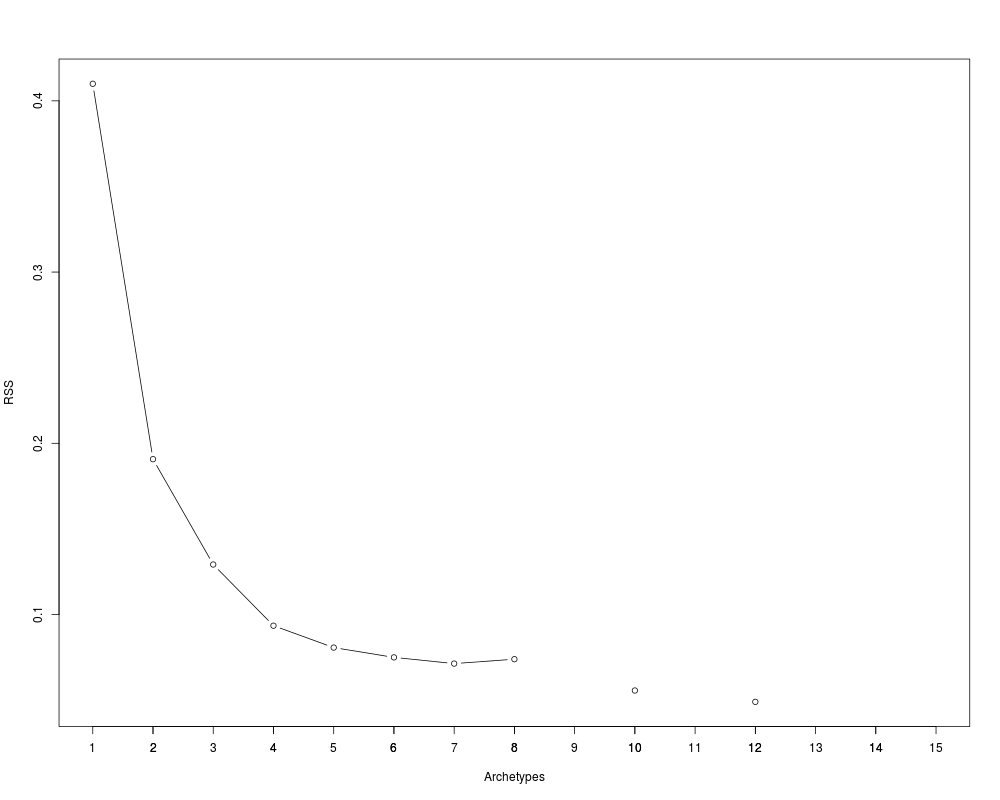
#Results shown in section 3.2 (figure 3):
screeplot(res) 

#3 archetypes:
a3 <- archetypes::bestModel(res[[3]])
archetypes::parameters(a3)
#7 archetypes:
a7 <- archetypes::bestModel(res[[7]])
archetypes::parameters(a7) 
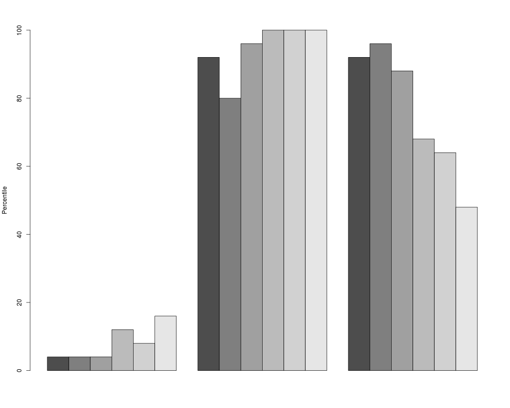
#Plotting the percentiles of each archetype:
#Figure 2 (b):
barplot(a3,USAFSurvey_preproc$data, percentiles = TRUE, which = "beside") 
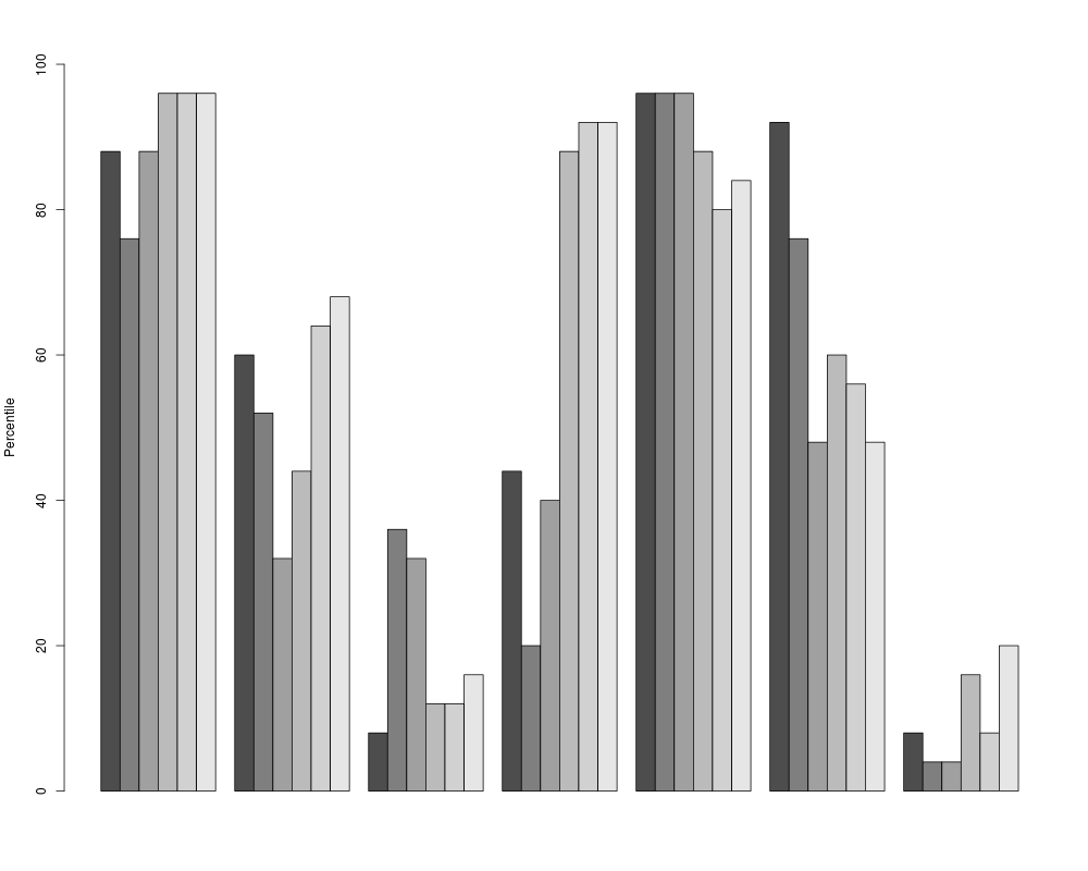
#Figure 2 (f):
barplot(a7,USAFSurvey_preproc$data, percentiles = TRUE, which = "beside")

#Results shown in section 3.3 related with PCA.
pznueva <- prcomp(USAFSurvey_preproc$data, scale = TRUE, retx = TRUE) 
#Table 3:
summary(pznueva)
pznueva
#PCA scores for 3 archetypes:
p3 <- predict(pznueva,archetypes::parameters(a3)) 
#PCA scores for 7 archetypes:
p7 <- predict(pznueva,archetypes::parameters(a7))
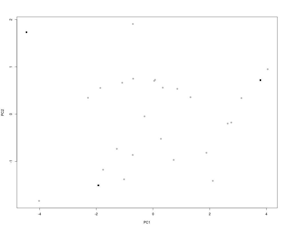
#Representing the scores:
#Figure 4 (a):
xyplotPCArchetypes(p3[,1:2], pznueva$x[,1:2], data.col = gray(0.7), atypes.col = 1, 
                   atypes.pch = 15)
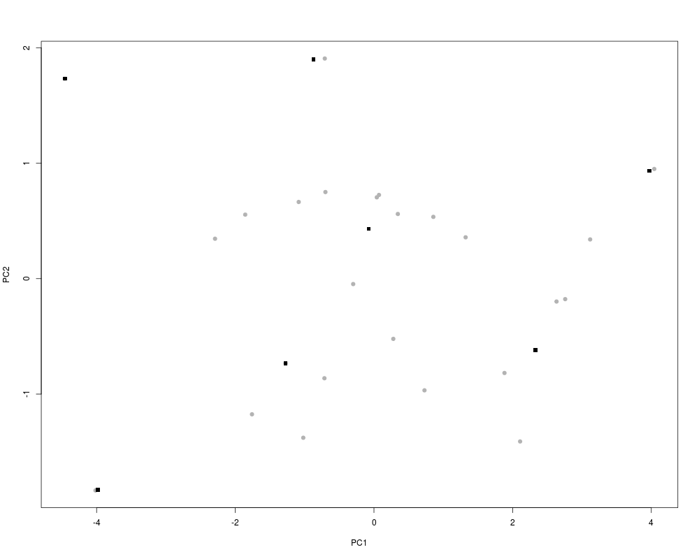
#Figure 4 (b):
xyplotPCArchetypes(p7[,1:2], pznueva$x[,1:2], data.col = gray(0.7), atypes.col = 1, 
                   atypes.pch = 15)

#Percentiles for 7 archetypes (table 5):
Fn <- ecdf(USAFSurvey_preproc$data)
round(Fn(archetypes::parameters(a7)) * 100)

#Which are the nearest individuals to archetypes?:
#Example for three archetypes:
ras <- rbind(archetypes::parameters(a3),USAFSurvey_preproc$data)
dras <- dist(ras,method = "euclidean", diag = FALSE, upper = TRUE, p = 2)
mdras <- as.matrix(dras)
diag(mdras) = 1e+11
numArch <- 3
sapply(seq(length=numArch),nearestToArchetypes,numArch,mdras) 

#In addition, we can turn the standardized values to the original variables.
p <- archetypes::parameters(a7)
m <- sapply(USAFSurvey_inch,mean)
s <- sapply(USAFSurvey_inch,sd)
d <- p
for(i in 1 : 6){
 d[,i] = p[,i] * s[i] + m[i]
}
#Table 7:
t(d)

Results


R version 3.3.1 (2016-06-21) -- "Bug in Your Hair"
Copyright (C) 2016 The R Foundation for Statistical Computing
Platform: x86_64-pc-linux-gnu (64-bit)

R is free software and comes with ABSOLUTELY NO WARRANTY.
You are welcome to redistribute it under certain conditions.
Type 'license()' or 'licence()' for distribution details.

R is a collaborative project with many contributors.
Type 'contributors()' for more information and
'citation()' on how to cite R or R packages in publications.

Type 'demo()' for some demos, 'help()' for on-line help, or
'help.start()' for an HTML browser interface to help.
Type 'q()' to quit R.

> library(Anthropometry)
> png(filename="/home/ddbj/snapshot/RGM3/R_CC/result/Anthropometry/archetypesBoundary.Rd_%03d_medium.png", width=480, height=480)
> ### Name: archetypesBoundary
> ### Title: Archetypal analysis in multivariate accommodation problem
> ### Aliases: archetypesBoundary
> ### Keywords: array
> 
> ### ** Examples
> 
> #The following R code allows us to reproduce the results of the paper Epifanio et al. (2013).
> #As a toy example, only the first 25 individuals are used.
> #First,the USAF 1967 database is read and preprocessed (Zehner et al. (1993)).
> #Variable selection:
> variabl_sel <- c(48, 40, 39, 33, 34, 36)
> #Changing to inches: 
> USAFSurvey_inch <- USAFSurvey[1:25, variabl_sel] / (10 * 2.54)
> 
> #Data preprocessing:
> USAFSurvey_preproc <- preprocessing(USAFSurvey_inch, TRUE, 0.95, TRUE)
[1] "The percentage of accommodation is exactly 100%"
> 
> #Procedure and results shown in section 2.2.2 and section 3.1:
> set.seed(2010)
> res <- archetypesBoundary(USAFSurvey_preproc$data, 15, FALSE, 3)
There were 32 warnings (use warnings() to see them)
> #To understand the warning messages, see the vignette of the
> #archetypes package.
> 
> #Results shown in section 3.2 (figure 3):
> screeplot(res) 
> 
> #3 archetypes:
> a3 <- archetypes::bestModel(res[[3]])
> archetypes::parameters(a3)
            V48        V40       V39        V33        V34       V36
[1,] -1.5270266 -1.9850068 -1.852909 -1.2017120 -1.4506087 -1.300550
[2,]  0.8587891  0.6344427  1.560531  3.0239130  2.7118268  1.936117
[3,]  1.2901837  1.5086416  1.377934  0.3089858  0.1200188  0.218374
> #7 archetypes:
> a7 <- archetypes::bestModel(res[[7]])
> archetypes::parameters(a7) 
             V48          V40         V39        V33         V34        V36
[1,]  0.85852864  0.634250226  1.56005808  3.0229958  2.71100419  1.9355296
[2,]  0.04305708 -0.001325421 -0.45533377 -0.1328833  0.13201106  0.6058085
[3,] -1.22857382 -0.362084645 -0.49526996 -1.2428477 -1.04775913 -1.2898170
[4,] -0.23418124 -0.796488173 -0.25947060  0.9076199  1.18207361  1.2022645
[5,]  2.62493417  2.122915205  2.38286566  0.9706358  0.84211796  0.9427605
[6,]  2.06013010  0.602315380 -0.03818875  0.2225773  0.06748302  0.2967602
[7,] -1.42616785 -2.321391279 -2.06151698 -1.1440309 -1.56690624 -1.2705278
> #Plotting the percentiles of each archetype:
> #Figure 2 (b):
> barplot(a3,USAFSurvey_preproc$data, percentiles = TRUE, which = "beside") 
> #Figure 2 (f):
> barplot(a7,USAFSurvey_preproc$data, percentiles = TRUE, which = "beside")
> 
> #Results shown in section 3.3 related with PCA.
> pznueva <- prcomp(USAFSurvey_preproc$data, scale = TRUE, retx = TRUE) 
> #Table 3:
> summary(pznueva)
Importance of components:
                          PC1    PC2     PC3     PC4     PC5     PC6
Standard deviation     2.0920 0.9724 0.60041 0.38492 0.36177 0.19582
Proportion of Variance 0.7294 0.1576 0.06008 0.02469 0.02181 0.00639
Cumulative Proportion  0.7294 0.8870 0.94710 0.97180 0.99361 1.00000
> pznueva
Standard deviations:
[1] 2.0920385 0.9723677 0.6004109 0.3849174 0.3617681 0.1958195

Rotation:
           PC1        PC2        PC3        PC4         PC5         PC6
V48 -0.3944472 -0.3205130 -0.7352829  0.2591028 -0.35919722  0.06989300
V40 -0.3866531 -0.5302035  0.1720589  0.2290238  0.67984717 -0.15854106
V39 -0.4064501 -0.3931392  0.4120171 -0.5569641 -0.41585880  0.16533074
V33 -0.4328513  0.3464121  0.2647274  0.2898743 -0.29714285 -0.67099683
V34 -0.4261090  0.3992454  0.2177968  0.3542715  0.05660779  0.69490001
V36 -0.4009738  0.4268477 -0.3774661 -0.6005576  0.37993201 -0.09758419
> #PCA scores for 3 archetypes:
> p3 <- predict(pznueva,archetypes::parameters(a3)) 
> #PCA scores for 7 archetypes:
> p7 <- predict(pznueva,archetypes::parameters(a7))
> #Representing the scores:
> #Figure 4 (a):
> xyplotPCArchetypes(p3[,1:2], pznueva$x[,1:2], data.col = gray(0.7), atypes.col = 1, 
+                    atypes.pch = 15)
> #Figure 4 (b):
> xyplotPCArchetypes(p7[,1:2], pznueva$x[,1:2], data.col = gray(0.7), atypes.col = 1, 
+                    atypes.pch = 15)
> 
> #Percentiles for 7 archetypes (table 5):
> Fn <- ecdf(USAFSurvey_preproc$data)
> round(Fn(archetypes::parameters(a7)) * 100)
 [1] 84 53 11 39 98 96  8 76 51 33 23 97 75  1 94 30 29 38 97 49  1 99 45 11 86
[26] 87 61 12 99 57 13 91 83 54  5 95 75 10 91 86 65 11
> 
> #Which are the nearest individuals to archetypes?:
> #Example for three archetypes:
> ras <- rbind(archetypes::parameters(a3),USAFSurvey_preproc$data)
> dras <- dist(ras,method = "euclidean", diag = FALSE, upper = TRUE, p = 2)
> mdras <- as.matrix(dras)
> diag(mdras) = 1e+11
> numArch <- 3
> sapply(seq(length=numArch),nearestToArchetypes,numArch,mdras) 
[1] 20  6  5
> 
> #In addition, we can turn the standardized values to the original variables.
> p <- archetypes::parameters(a7)
> m <- sapply(USAFSurvey_inch,mean)
> s <- sapply(USAFSurvey_inch,sd)
> d <- p
> for(i in 1 : 6){
+  d[,i] = p[,i] * s[i] + m[i]
+ }
> #Table 7:
> t(d)
        [,1]     [,2]     [,3]     [,4]     [,5]     [,6]     [,7]
V48 34.25183 32.67836 30.22470 32.14342 37.66017 36.57036 29.84344
V40 24.80309 24.05040 23.62316 23.10872 26.56606 24.76527 21.30283
V39 18.66129 16.57615 16.53484 16.77879 19.51257 17.00773 14.91439
V33 41.25950 36.82263 35.26212 38.28548 38.37407 37.32237 35.40105
V34 35.43281 32.32147 30.89817 33.58828 33.17815 32.24362 30.27186
V36 26.45652 24.95496 22.81437 25.62849 25.33546 24.60598 22.83615
> 
> 
> 
> 
> 
> dev.off()
null device 
          1 
>