A character vector, with names of variables. The first block of
independent variables.
...
A character vector, with names of variables. Subsequent blocks of
independent variables.
dataset
A data frame containing variables refered to in
formulas, passed to data argument of lm
type
Family argument to pass to glm. Specify "binomial" for
binary logistic regression models.
assumptions.check
Boolean, if TRUE, then assumption checks are run and
output is produced. If FALSE, only model summary and coefficient tables are
produced.
outliers.check
Determines how many observations to display for
outliers check. Default is significant observations. "All" shows all
residual and Cook's D values.
transform.outcome
A boolean. If TRUE, a variable transformation of the
outcome is substituted in the final model if outcome is non-normal. NOT
IMPLEMENTED YET.
Details
Calls other functions to generate model objects and test them, given
specified model parameters and other options. Formatted output is produced
via model_output
R version 3.3.1 (2016-06-21) -- "Bug in Your Hair"
Copyright (C) 2016 The R Foundation for Statistical Computing
Platform: x86_64-pc-linux-gnu (64-bit)
R is free software and comes with ABSOLUTELY NO WARRANTY.
You are welcome to redistribute it under certain conditions.
Type 'license()' or 'licence()' for distribution details.
R is a collaborative project with many contributors.
Type 'contributors()' for more information and
'citation()' on how to cite R or R packages in publications.
Type 'demo()' for some demos, 'help()' for on-line help, or
'help.start()' for an HTML browser interface to help.
Type 'q()' to quit R.
> library(AutoModel)
> png(filename="/home/ddbj/snapshot/RGM3/R_CC/result/AutoModel/run_model.Rd_%03d_medium.png", width=480, height=480)
> ### Name: run_model
> ### Title: Automated Multiple Regression Modelling
> ### Aliases: run_model
>
> ### ** Examples
>
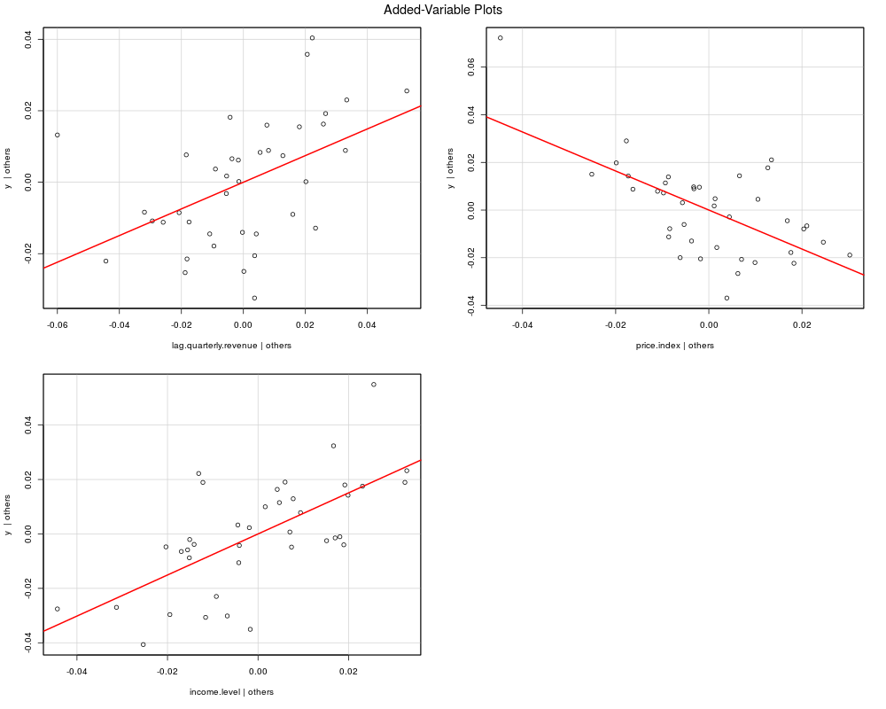
> run_model("y", c("lag.quarterly.revenue"), c("price.index", "income.level"),
+ dataset=freeny)
REGRESSION OUTPUT
Durbin-Watson = 2.11 p value = 0.4729
Partial Regression plots (all relationships should be linear):
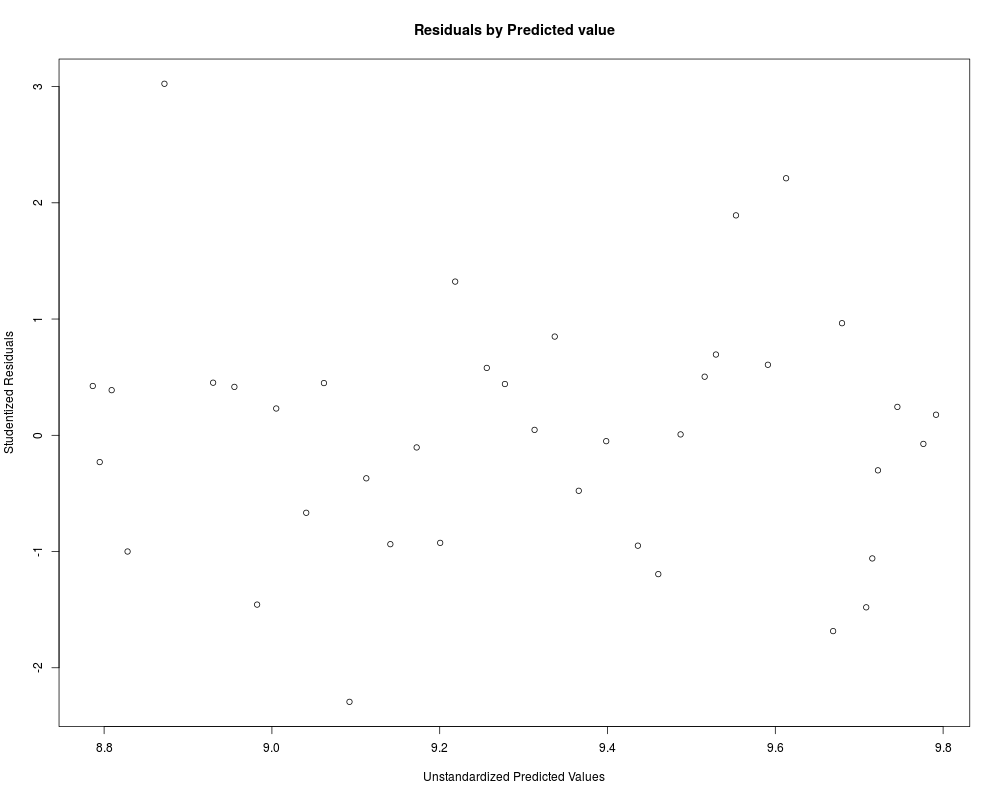
Plot of studentized residuals: uniform distibution across predicted values requiredCorrelation Matrix for model (correlation >.70 indicates severe multicollinearity)
y lag.quarterly.revenue price.index income.level
y 1.0000 0.9978 -0.9895 0.9839
lag.quarterly.revenue 0.9978 1.0000 -0.9894 0.9817
price.index -0.9895 -0.9894 1.0000 -0.9539
income.level 0.9839 0.9817 -0.9539 1.0000
Variance inflation factor (<10 desired):
lag.quarterly.revenue price.index income.level
194.85 78.58 45.52
Standardized Residuals (observations > 3.00 problematic):
No significant outliers
Cook's distance (values >.2 problematic):
1963.25
0.8918
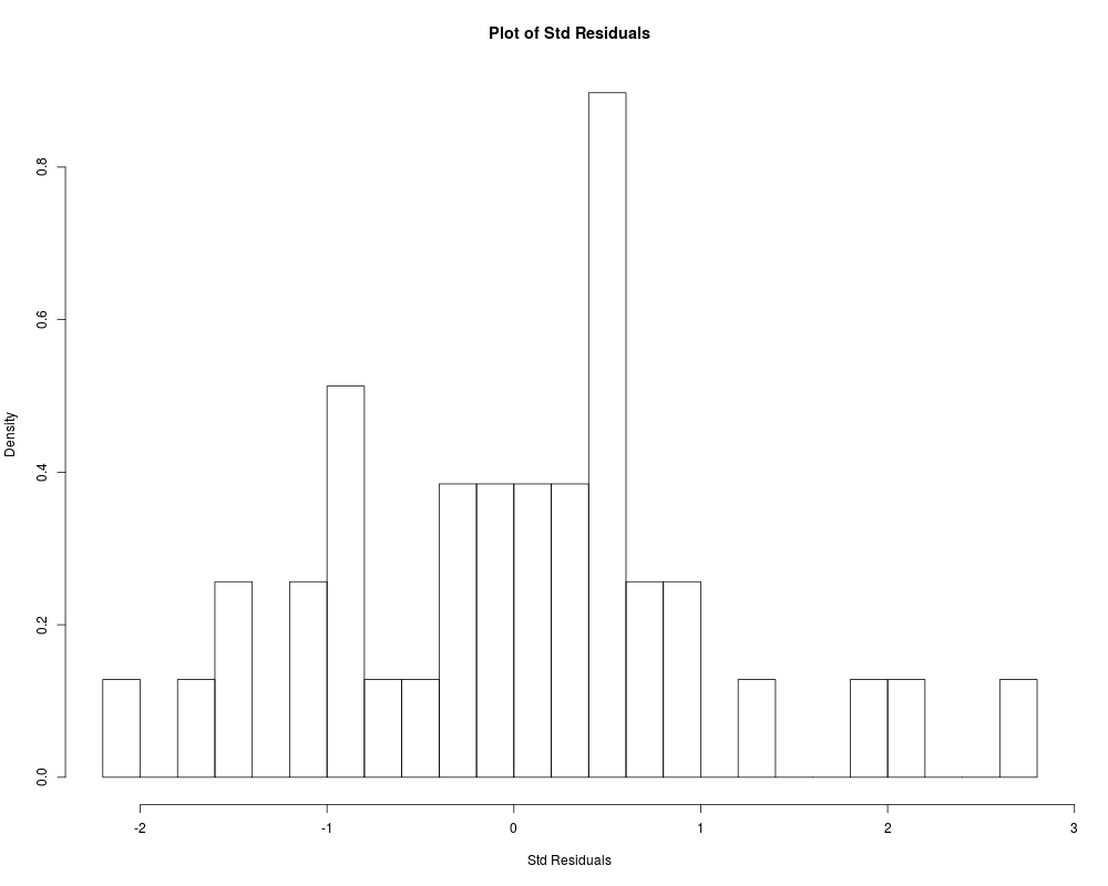
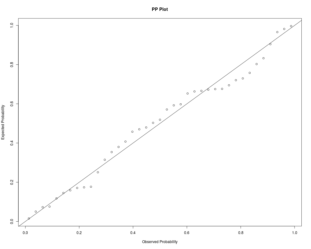
Normality of standardized model residuals: Shapiro-Wilk (p-value): 0.5586
Model change statistics
R R^2 Adj R^2 SE Est. Delta R^2 F Change df1 df2 p Fch Sig
Model 1 0.9978 0.9956 0.9955 0.0212 0.9956 8360.3793 1 37 0 ***
Model 2 0.9988 0.9977 0.9975 0.0159 0.0021 15.4599 2 35 0 ***
Model 1 : y ~ lag.quarterly.revenue
Model 2 : y ~ lag.quarterly.revenue + price.index + income.level
Model Coefficients
Model term estimate std.error statistic p.value sig
Model 1 (Intercept) 0.04169 0.10138 0.4112 0.6833
Model 1 lag.quarterly.revenue 0.99827 0.01092 91.4351 0.0000 ***
Model 2 (Intercept) 4.97077 1.24046 4.0072 0.0003 ***
Model 2 lag.quarterly.revenue 0.37305 0.11418 3.2673 0.0024 **
Model 2 price.index -0.81887 0.17152 -4.7742 0.0000 ***
Model 2 income.level 0.75435 0.14454 5.2189 0.0000 ***
>
>
>
>
>
> dev.off()
null device
1
>
 .
.