R: A graphical tool to visualize and compare functional...
BACA-package
R Documentation
A graphical tool to visualize and compare functional annotations retrieved from DAVID knowledgebase.
Description
DAVID Bioinformatics Resources (DAVID) at http://david.abcc.ncifcrf.gov is the most popular tool in functional annotation and enrichment analysis. It provides an integrated biological knowledgebase and tools to systematically extract relevant biological terms (e.g., GO terms, KEGG pathways) associated with a given gene list. After submitting a gene list, DAVID annotation tool finds the most enriched annotations and presents them in a table format. This table contains many different types of data, such as text, numbers, bars and hyperlinks, that can be hard tor read and compare when multiple enrichment results are available. The BACA package tries to address these issues by providing a novel R-based graphical tool to concisely visualize DAVID annotations and show how they change across different experimental conditions. This R package uses some functions available in the R package RDAVIDWebService available at http://www.bioconductor.org/packages/release/bioc/html/RDAVIDWebService.html.
Details
Package:
BACA
Type:
Package
Version:
1.0
Date:
2014-06-19
License:
GPL (>=2)
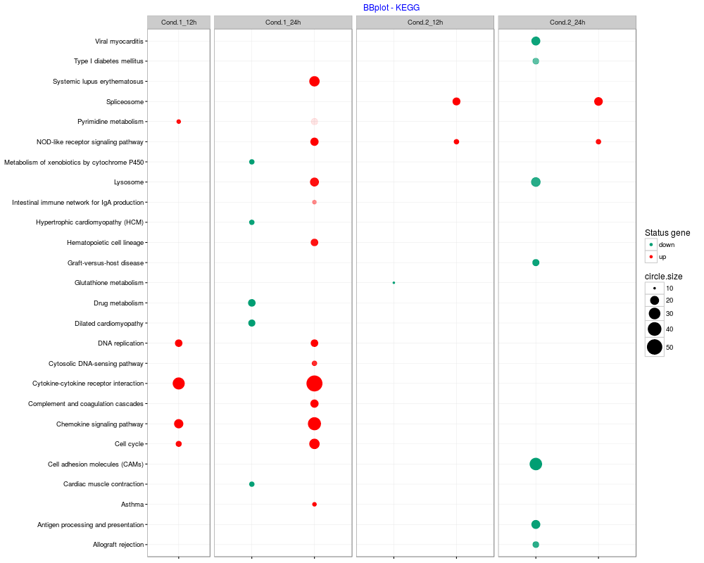
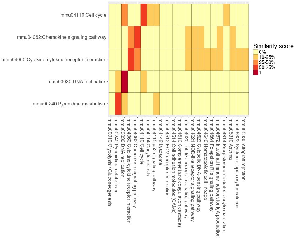
The package BACA provides three different functions: DAVIDsearch, BBplot and Jplot. DAVIDsearch: to call the Functional Annotation Tool of DAVID. BBplot: to build a grid where each row represents an enriched annotation found by DAVID and each column the condition/treatment where that annotation was highlighted. While, each cell reports a bubble indicating the number of genes enriching the correpsonding annotation and the state of these genes in terms of down- and up-regulation (default setting: green = "down" - red = "up"). Jplot: to make a table/matrix with colored boxes. The color of each box indicated the Jaccard index based similarity score calculated between the genes sets associated with two different functional annotations.
R version 3.3.1 (2016-06-21) -- "Bug in Your Hair"
Copyright (C) 2016 The R Foundation for Statistical Computing
Platform: x86_64-pc-linux-gnu (64-bit)

R is free software and comes with ABSOLUTELY NO WARRANTY.
You are welcome to redistribute it under certain conditions.
Type 'license()' or 'licence()' for distribution details.

R is a collaborative project with many contributors.
Type 'contributors()' for more information and
'citation()' on how to cite R or R packages in publications.

Type 'demo()' for some demos, 'help()' for on-line help, or
'help.start()' for an HTML browser interface to help.
Type 'q()' to quit R.

> library(BACA)

> png(filename="/home/ddbj/snapshot/RGM3/R_CC/result/BACA/BACA-package.Rd_%03d_medium.png", width=480, height=480)
> ### Name: BACA-package
> ### Title: A graphical tool to visualize and compare functional annotations
> ###   retrieved from DAVID knowledgebase.
> ### Aliases: BACA-package BACA
>
> ### ** Examples
>
>   data(result.kegg)
>
>   bbplot.kegg <- BBplot(result.kegg, max.pval = 0.05, min.ngenes = 10,
+                     name.com = c("Cond.1_12h","Cond.1_24h","Cond.2_12h","Cond.2_24h"),
+                     labels = c("down", "up"), colors = c("#009E73", "red"),
+                     title = "BBplot - KEGG", print.term = "description")
>   bbplot.kegg
>   ##ggsave("KEGG_terms.tiff", width=6, height=4, scale=2, dpi=200)
>
>   jplot.kegg <- Jplot(result.kegg[[4]], result.kegg[[2]], max.pval = 0.05, min.ngenes = 10)
>
>   jplot.kegg
>   ##ggsave("j_plot.tiff", width=6, height=4, scale=2, dpi=200)
>
>
>
>
>
> dev.off()
null device
          1
>
 .
.