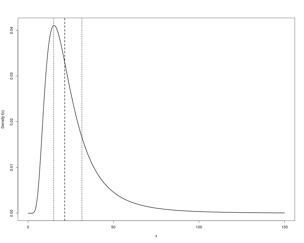
The Gamma-Gamma Distribution

Description

Density and random generation for the Gamma-Gamma distribution with parameters shape1, rate1, and shape2.

Usage

  dggamma(x, shape1, rate1, shape2)
  rggamma(n, shape1, rate1, shape2)

Arguments

Details

A Gamma-Gamma distribution with parameters shape1 = a, rate1 = r and shape2 = b has density

f(x) = [(r^a)/(Gamma(a))][Gamma(a+b)/Gamma(b)] [x^(b-1)/(r+x)^(a+b)]

for x > 0 where a,r > 0 and b = 1,2,….

The distribution is generated using the following scheme:

1. Generate Y ~ Gamma(shape=shape1,rate=rate1).

2. Generate X ~ Gamma(shape=shape2,rate=Y).

Then, X follows a Gamma-Gamma distribution.

Value

dggamma gives the density, and rggamma gives random variates.

References

Bernardo JM, Smith AFM. (1994) Bayesian Theory. Wiley, New York.

See Also

dgamma

Examples

############################################################
# Construct a plot of the density function with median and
# quantiles marked.

# define parameters
shape1 <- 4
rate1 <- 4
shape2 <- 20

# construct density plot
x <- seq(0.1,150,0.1)
plot(dggamma(x,shape1,rate1,shape2)~x,
     type="l",lwd=2,main="",xlab="x",ylab="Density f(x)")
     
# determine median and quantiles
set.seed(123)
X <- rggamma(5000,shape1,rate1,shape2)
quants <- quantile(X,prob=c(0.25,0.5,0.75))

# add quantities to plot
abline(v=quants,lty=c(3,2,3),lwd=2)


############################################################
# Consider the following set-up:
#   Let x ~ N(theta,sigma2), sigma2 is unknown variance.
#   Consider a prior on theta and sigma2 defined by
#      theta|sigma2 ~ N(mu,(r*sigma)^2)
#      sigma2 ~ InverseGamma(a/2,b/2), (b/2) = rate.
#
#   We want to generate random variables from the marginal
#   (prior predictive) distribution of the sufficient
#   statistic T = (xbar,s2) where the sample size n = 25.

# define parameters
a <- 4
b <- 4
mu <- 1 
r <- 3
n <- 25


# generate random variables from Gamma-Gamma
set.seed(123)
shape1 <- a/2
rate1 <- b
shape2 <- 0.5*(n-1)

Y <- rggamma(5000,shape1,rate1,shape2)

# generate variables from a non-central t given Y
df <- n+a-1
scale <- (Y+b)*(1/n + r^2)/(n+a-1)

X <- rt(5000,df=df)*sqrt(scale) + mu

# the pair (X,Y) comes from the correct marginal density

# mean of xbar and s2, and xbar*s2
mean(X)
mean(Y)
mean(X*Y)

Results

R version 3.3.1 (2016-06-21) -- "Bug in Your Hair"
Copyright (C) 2016 The R Foundation for Statistical Computing
Platform: x86_64-pc-linux-gnu (64-bit)

R is free software and comes with ABSOLUTELY NO WARRANTY.
You are welcome to redistribute it under certain conditions.
Type 'license()' or 'licence()' for distribution details.

R is a collaborative project with many contributors.
Type 'contributors()' for more information and
'citation()' on how to cite R or R packages in publications.

Type 'demo()' for some demos, 'help()' for on-line help, or
'help.start()' for an HTML browser interface to help.
Type 'q()' to quit R.

> library(BAEssd)
Loading required package: mvtnorm
> png(filename="/home/ddbj/snapshot/RGM3/R_CC/result/BAEssd/GammaGamma.Rd_%03d_medium.png", width=480, height=480)
> ### Name: GammaGamma
> ### Title: The Gamma-Gamma Distribution
> ### Aliases: GammaGamma dggamma rggamma
> 
> ### ** Examples
> 
> ############################################################
> # Construct a plot of the density function with median and
> # quantiles marked.
> 
> # define parameters
> shape1 <- 4
> rate1 <- 4
> shape2 <- 20
> 
> # construct density plot
> x <- seq(0.1,150,0.1)
> plot(dggamma(x,shape1,rate1,shape2)~x,
+      type="l",lwd=2,main="",xlab="x",ylab="Density f(x)")
>      
> # determine median and quantiles
> set.seed(123)
> X <- rggamma(5000,shape1,rate1,shape2)
> quants <- quantile(X,prob=c(0.25,0.5,0.75))
> 
> # add quantities to plot
> abline(v=quants,lty=c(3,2,3),lwd=2)
> 
> 
> ############################################################
> # Consider the following set-up:
> #   Let x ~ N(theta,sigma2), sigma2 is unknown variance.
> #   Consider a prior on theta and sigma2 defined by
> #      theta|sigma2 ~ N(mu,(r*sigma)^2)
> #      sigma2 ~ InverseGamma(a/2,b/2), (b/2) = rate.
> #
> #   We want to generate random variables from the marginal
> #   (prior predictive) distribution of the sufficient
> #   statistic T = (xbar,s2) where the sample size n = 25.
> 
> # define parameters
> a <- 4
> b <- 4
> mu <- 1 
> r <- 3
> n <- 25
> 
> 
> # generate random variables from Gamma-Gamma
> set.seed(123)
> shape1 <- a/2
> rate1 <- b
> shape2 <- 0.5*(n-1)
> 
> Y <- rggamma(5000,shape1,rate1,shape2)
> 
> # generate variables from a non-central t given Y
> df <- n+a-1
> scale <- (Y+b)*(1/n + r^2)/(n+a-1)
> 
> X <- rt(5000,df=df)*sqrt(scale) + mu
> 
> # the pair (X,Y) comes from the correct marginal density
> 
> # mean of xbar and s2, and xbar*s2
> mean(X)
[1] 0.9701382
> mean(Y)
[1] 51.11077
> mean(X*Y)
[1] 9.203261
> 
> 
> 
> 
> 
> dev.off()
null device 
          1 
>