R Graphical Manual

Browse All

Last data update: 2014.03.03

R: Binomial Suite: One Sample, One Sided

binom1.1sided

R Documentation

Binomial Suite: One Sample, One Sided

Description

Generates the suite of functions related to the one sample binomial experiment with a one-sided alternative hypothesis of interest.

Usage

  binom1.1sided(p0, a, b)

Arguments

`p0`	Scalar. The upper bound of p under null hypothesis Ho: p<=p0.
`a`	Scalar. Shape1 parameter for prior Beta distribution. See documentation for `dbeta`.
`b`	Scalar. Shape2 parameter for prior Beta distribution. See documentation for `dbeta`.

Details

binom1.1sided is used to generate a suite of functions for a one-sample binomial experiment with a one-sided alternative hypothesis. That is, when

X ~ Binomial(n,p)

H0: p <= p0 vs. H1: p > p0

using the following prior on p

p ~ Beta(a,b).

The functions that are generated are useful in examining the prior and posterior densities of the parameter p, as well as constructing the Bayes Factor and determining the sample size via an average error based approach.

The arguments of binom1.1sided are passed to each of the additional functions upon their creation as default values. That is, if p0 is set to 0.5 in the call to binom1.1sided, each of the functions returned will have the defaualt value of 0.5 for p0. If an argument is not specified in the call to binom1.1sided, then it remains a required parameter in all functions created.

Value

binom1.1sided returns a list of 4 functions. These functions are useful for either visualizing the problem, or computing the required sample size:

`logm`	The function returns a list of three vectors: the log marginal density under the null hypothesis (`logm0`), the log marginal density under the alternative hypothesis (`logm1`), and the log marginal density (`logm`). Each are evaluated at the observed data provided. This function is also passed to `ssd.binom` to calculate required sample sizes. This function has the following usage: logm(x, n, p0, a, b) `x`: Vector. Number of successes observed, out of `n` independent Bernoulli trials. `n`: Scalar. Sample size, the number of independent Bernoulli trials. Remaining parameters are specified above for `binom1.1sided`.
`logbf`	Returns a vector: the value of the log Bayes Factor given the observed data provided and the prior parameters specified. This function has the following usage: logbf(x, n, p0, a, b) For details on the parameters for this function, see the above description for `logm`.
`prior`	Returns a vector: the value of the prior density at the specified value of `p` with parameters `a` and `b`. This function has the following usage: prior(p, a, b) `p`: Vector. Quantiles at which to evaluate the prior distribution. Remaining parameters are specified above for `binom1.1sided`.
`post`	Returns a vector: the value of the posterior density. This function has the following usage: post(p, x, n, a, b) `p`: Vector. Quantiles at which to evaluate the posterior distribution. `x`: Scalar. Number of successes observed, out of `n` independent Bernoulli trials. `n`: Scalar: The number of independent Bernoulli trials. Remaining parameters are specified above for `binom1.1sided`.

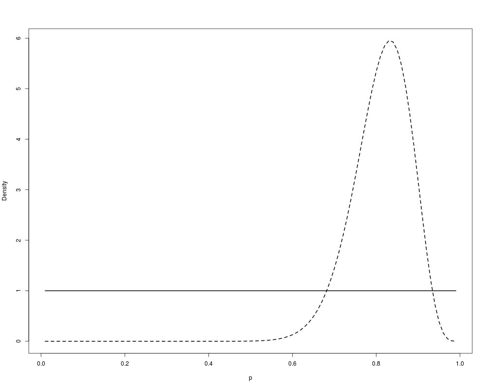
Examples

############################################################
# Generate the suite of functions for a one-sample binomial
# with a one-sided test. Consider the hypothesis
#      H0: p<=0.5   vs.  H1: p>0.5
#
# with a uniform prior on p.

# generate suite
f1 <- binom1.1sided(p0=0.5,a=1,b=1)

# attach suite
attach(f1)

# plot prior and posterior given x = 25, n = 30
ps <- seq(0.01,0.99,0.01)
p1 <- prior(ps)
p2 <- post(ps,x=25,n=30)

plot(c(p1,p2)~rep(ps,2),type="n",ylab="Density",xlab="p",main="")
lines(p1~ps,lty=1,lwd=2)
lines(p2~ps,lty=2,lwd=2)

# perform sample size calculation with TE bound of 0.25 and weight 0.5
ssd.binom(alpha=0.25,w=0.5,logm=logm)

# detain suite
detach(f1)

Results


R version 3.3.1 (2016-06-21) -- "Bug in Your Hair"
Copyright (C) 2016 The R Foundation for Statistical Computing
Platform: x86_64-pc-linux-gnu (64-bit)

R is free software and comes with ABSOLUTELY NO WARRANTY.
You are welcome to redistribute it under certain conditions.
Type 'license()' or 'licence()' for distribution details.

R is a collaborative project with many contributors.
Type 'contributors()' for more information and
'citation()' on how to cite R or R packages in publications.

Type 'demo()' for some demos, 'help()' for on-line help, or
'help.start()' for an HTML browser interface to help.
Type 'q()' to quit R.

> library(BAEssd)
Loading required package: mvtnorm
> png(filename="/home/ddbj/snapshot/RGM3/R_CC/result/BAEssd/binom1.1sided.Rd_%03d_medium.png", width=480, height=480)
> ### Name: binom1.1sided
> ### Title: Binomial Suite: One Sample, One Sided
> ### Aliases: binom1.1sided
> 
> ### ** Examples
> 
> ############################################################
> # Generate the suite of functions for a one-sample binomial
> # with a one-sided test. Consider the hypothesis
> #      H0: p<=0.5   vs.  H1: p>0.5
> #
> # with a uniform prior on p.
> 
> # generate suite
> f1 <- binom1.1sided(p0=0.5,a=1,b=1)

Loading the 'binom1.1sided' suite... 
  This suite contains functions pertaining to a one sample experiment 
  with a binary outcome. The hypothesis of interest has a one-sided 
  alternative.

> 
> # attach suite
> attach(f1)
> 
> # plot prior and posterior given x = 25, n = 30
> ps <- seq(0.01,0.99,0.01)
> p1 <- prior(ps)
> p2 <- post(ps,x=25,n=30)
> 
> plot(c(p1,p2)~rep(ps,2),type="n",ylab="Density",xlab="p",main="")
> lines(p1~ps,lty=1,lwd=2)
> lines(p2~ps,lty=2,lwd=2)
> 
> # perform sample size calculation with TE bound of 0.25 and weight 0.5
> ssd.binom(alpha=0.25,w=0.5,logm=logm)

Bayesian Average Error Sample Size Determination

Call: ssd.binom(alpha = 0.25, w = 0.5, logm = logm)

Sample Size:  9
Total Average Error:  0.2460938

Acceptable sample size determined!

> 
> # detain suite
> detach(f1)
> 
> 
> 
> 
> 
> dev.off()
null device 
          1 
>