Supported by Dr. Osamu Ogasawara and  . . |
|
Last data update: 2014.03.03 |
Binomial Suite: One Sample, Two SidedDescriptionGenerates the suite of functions related to the one sample binomial experiment with a two-sided alternative hypothesis of interest. Usagebinom1.2sided(p0, prob, a, b) Arguments
Details
X ~ Binomial(n,p) H0: p == p0 vs. H1: p != p0 using the following prior on p pi(p) = u*(p==p0) + (1-u)*(p!=p0)Beta(a,b), where Beta(a,b) is Beta density with parameters The functions that are generated are useful in examining the prior and
posterior densities of the parameter The arguments of Value
See Also
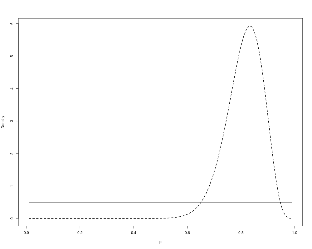
Examples############################################################ # Generate the suite of functions for a one-sample binomial # with a two-sided test. Consider the hypothesis # H0: p==0.5 vs. H1: p!=0.5 # # with a uniform prior on p under the alternative and a # prior probability of the null hypothesis equal to 0.5. # generate suite f2 <- binom1.2sided(p0=0.5,prob=0.5,a=1,b=1) # attach suite attach(f2) # plot prior and posterior given x = 25, n = 30 # - don't forget that point mass is not shown on plot ps <- seq(0.01,0.99,0.01) p1 <- prior(ps) p2 <- post(ps,x=25,n=30) plot(c(p1,p2)~rep(ps,2),type="n",ylab="Density",xlab="p",main="") lines(p1~ps,lty=1,lwd=2) lines(p2~ps,lty=2,lwd=2) # perform sample size calculation with TE bound of 0.25 and weight 0.5 ssd.binom(alpha=0.25,w=0.5,logm=logm) # detain suite detach(f2) Results
R version 3.3.1 (2016-06-21) -- "Bug in Your Hair"
Copyright (C) 2016 The R Foundation for Statistical Computing
Platform: x86_64-pc-linux-gnu (64-bit)

R is free software and comes with ABSOLUTELY NO WARRANTY.
You are welcome to redistribute it under certain conditions.
Type 'license()' or 'licence()' for distribution details.

R is a collaborative project with many contributors.
Type 'contributors()' for more information and
'citation()' on how to cite R or R packages in publications.

Type 'demo()' for some demos, 'help()' for on-line help, or
'help.start()' for an HTML browser interface to help.
Type 'q()' to quit R.

> library(BAEssd)
Loading required package: mvtnorm
> png(filename="/home/ddbj/snapshot/RGM3/R_CC/result/BAEssd/binom1.2sided.Rd_%03d_medium.png", width=480, height=480)
> ### Name: binom1.2sided
> ### Title: Binomial Suite: One Sample, Two Sided
> ### Aliases: binom1.2sided
>
> ### ** Examples
>
> ############################################################
> # Generate the suite of functions for a one-sample binomial
> # with a two-sided test. Consider the hypothesis
> #      H0: p==0.5   vs.  H1: p!=0.5
> #
> # with a uniform prior on p under the alternative and a
> # prior probability of the null hypothesis equal to 0.5.
>
> # generate suite
> f2 <- binom1.2sided(p0=0.5,prob=0.5,a=1,b=1)

Loading the 'binom1.2sided' suite...
  This suite contains functions pertaining to a one sample experiment
  with a binary outcome. The hypothesis of interest has a two-sided
  alternative.

>
> # attach suite
> attach(f2)
>
> # plot prior and posterior given x = 25, n = 30
> #  - don't forget that point mass is not shown on plot
> ps <- seq(0.01,0.99,0.01)
> p1 <- prior(ps)
> p2 <- post(ps,x=25,n=30)
>
> plot(c(p1,p2)~rep(ps,2),type="n",ylab="Density",xlab="p",main="")
> lines(p1~ps,lty=1,lwd=2)
> lines(p2~ps,lty=2,lwd=2)
>
> # perform sample size calculation with TE bound of 0.25 and weight 0.5
> ssd.binom(alpha=0.25,w=0.5,logm=logm)

Bayesian Average Error Sample Size Determination

Call: ssd.binom(alpha = 0.25, w = 0.5, logm = logm)

Sample Size:  94
Total Average Error:  0.2494501

Acceptable sample size determined!

>
> # detain suite
> detach(f2)
>
>
>
>
>
> dev.off()
null device
          1
>
|