Create plots of various average errors as a function of the sample size
calculated via the Bayesian Average Error based approach.
Usage
  ## S3 method for class 'BAEssd'
plot(x, y = "TE", alpha.line = TRUE, type = "l",
    xlab = "Sample Size (n)", ylab = NULL, main = NULL, ...)
Arguments
x
BAEssd object. Result from a Bayesian Average Error based sample size
calculation.
y
Character string. Indicates what type of error should be plotted on the
y-axis (default being Total Error). One of "TE","TWE","AE1", or "AE2".
alpha.line
Boolean. If TRUE, a horizontal line - indicating the bound on Total
Error used in determining the sample size - is added to the plot.
type, xlab, ylab, main
Character string. See plot.default() for more details.
...
Additional parameters to be passed to plotting functions.
Details
Each BAEssd object contains a history of the Average Errors for each
sample size considered. plot.BAEssd allows for examination of the
trend in errors as the sample size changes.
See Also
ssd, plot.default
Examples
############################################################
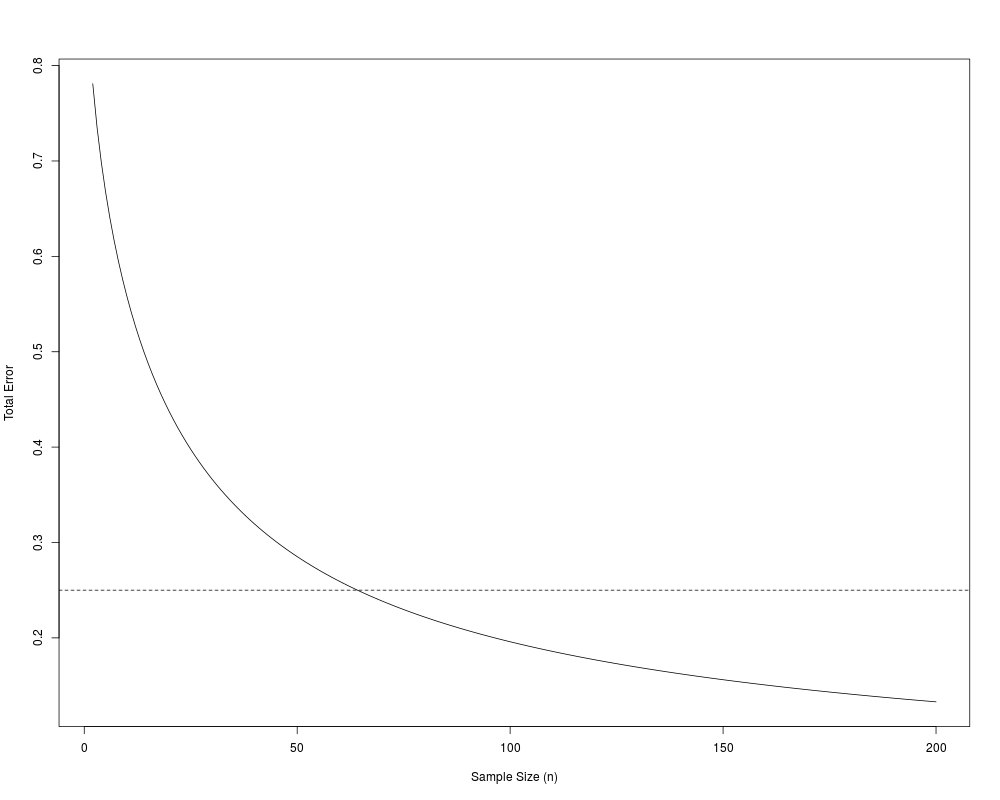
# Construct a plot of the Total Error as a function of
# sample size for a one-sample normal experiment with known
# variance.
# load suite of functions
f1 <- norm1KV.2sided(sigma=5,theta0=0,prob=0.5,mu=2,tau=1)
# get TE for many more sample sizes larger than the optimal
attach(f1)
ss1 <- ssd.norm1KV.2sided(alpha=0.25,w=0.5,minn=2,maxn=200,all=TRUE)
ss1
detach(f1)
# create plot of Total Error
plot(ss1)
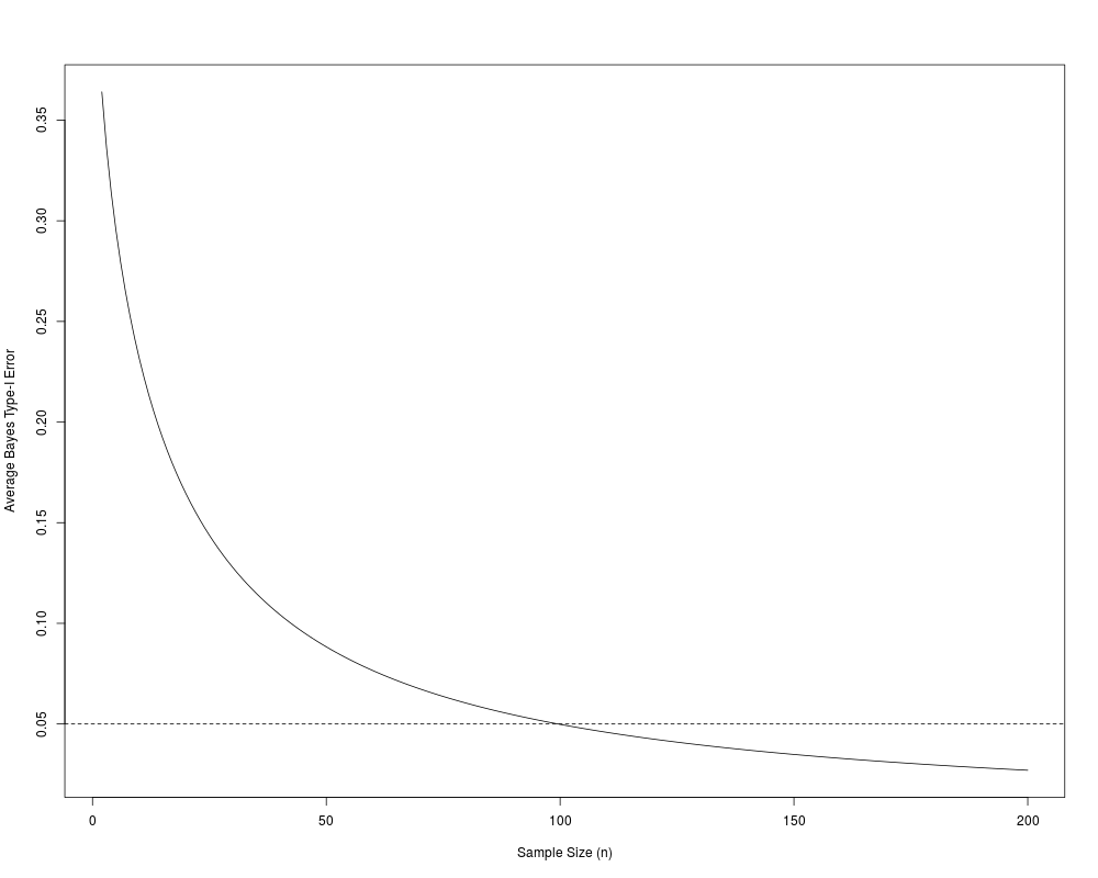
# create plot of Average Type-I Error
plot(ss1,y="AE1",alpha.line=FALSE)
abline(h=0.05,lty=2)
Results
R version 3.3.1 (2016-06-21) -- "Bug in Your Hair"
Copyright (C) 2016 The R Foundation for Statistical Computing
Platform: x86_64-pc-linux-gnu (64-bit)

R is free software and comes with ABSOLUTELY NO WARRANTY.
You are welcome to redistribute it under certain conditions.
Type 'license()' or 'licence()' for distribution details.

R is a collaborative project with many contributors.
Type 'contributors()' for more information and
'citation()' on how to cite R or R packages in publications.

Type 'demo()' for some demos, 'help()' for on-line help, or
'help.start()' for an HTML browser interface to help.
Type 'q()' to quit R.

> library(BAEssd)
Loading required package: mvtnorm
> png(filename="/home/ddbj/snapshot/RGM3/R_CC/result/BAEssd/plot.BAEssd.Rd_%03d_medium.png", width=480, height=480)
> ### Name: plot.BAEssd
> ### Title: Plotting Average Errors
> ### Aliases: plot.BAEssd
>
> ### ** Examples
>
> ############################################################
> # Construct a plot of the Total Error as a function of
> # sample size for a one-sample normal experiment with known
> # variance.
>
> # load suite of functions
> f1 <- norm1KV.2sided(sigma=5,theta0=0,prob=0.5,mu=2,tau=1)

Loading the 'norm1KV.2sided' suite...
  This suite contains functions pertaining to one-sample experiment
  involving a normally distributed response with known variance. The
  hypothesis of interest has a two-sided alternative.

>
> # get TE for many more sample sizes larger than the optimal
> attach(f1)
> ss1 <- ssd.norm1KV.2sided(alpha=0.25,w=0.5,minn=2,maxn=200,all=TRUE)
> ss1

Bayesian Average Error Sample Size Determination

Call: ssd.norm1KV.2sided(alpha = 0.25, w = 0.5, minn = 2, maxn = 200,
    all = TRUE)

Sample Size:  65
Total Average Error:  0.2482418

Acceptable sample size determined!

> detach(f1)
>
> # create plot of Total Error
> plot(ss1)
>
> # create plot of Average Type-I Error
> plot(ss1,y="AE1",alpha.line=FALSE)
> abline(h=0.05,lty=2)
>
>
>
>
>
> dev.off()
null device
          1
>
 .
.