Branch-specific rate shift probabilities

Description

marginalShiftProbsTree computes a version of a phylogenetic tree where each branch length is equal to the marginal probability that a shift occurred on a particular branch. The cumulativeShiftProbsTree includes the cumulative probability that a shift occurred on a given branch. See details.

Usage

cumulativeShiftProbsTree(ephy)

marginalShiftProbsTree(ephy)

Arguments

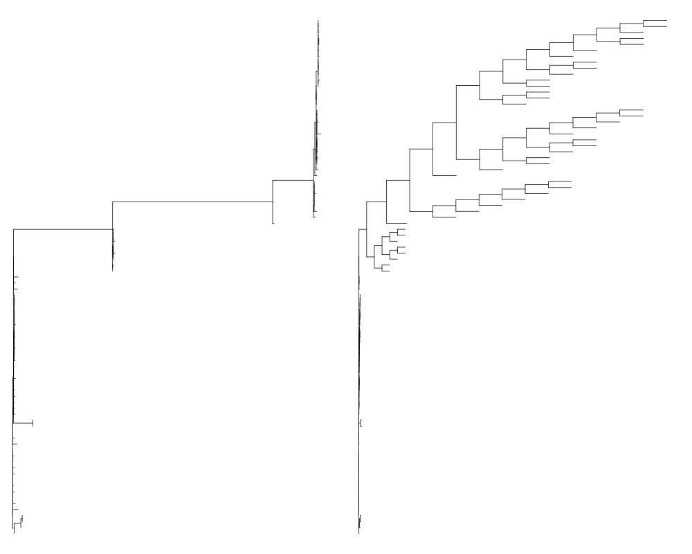
Details

The marginal shift probability tree is a copy of the target phylogeny, but where each branch length is equal to the branch-specific marginal probability that a rate-shift occurred on the focal branch. For example, a branch length of 0.333 implies that 1/3 of all samples from the posterior had a rate shift on the focal branch.

Note: It is highly inaccurate to use marginal shift probabilities as a measure of whether diversification rate heterogeneity occurs within a given dataset. Consider the following example. Suppose you have a tree with topology (A, (B, C)). You find a marginal shift probability of 0.5 on the branch leading to clade C, and also a marginal shift probability of 0.5 on the branch leading to clade BC. Even though the marginal shift probabilities appear low, it may be the case that the joint probability of a shift occurring on either the branch leading to C or BC is 1.0. Hence, you could be extremely confident (posterior probabilities approaching 1.0) in rate heterogeneity, yet find that no single branch has a particularly high marginal shift probability. In fact, this is exactly what we expect in most real datasets, because there is rarely enough signal to strongly support the occurrence of a shift on any particular branch.

The cumulative shift probability tree is a copy of the target phylogeny but where branch lengths are equal to the cumulative probability that a rate shift occurred somewhere on the path between the root and the focal branch. A branch length equal to 0.0 implies that the branch in question has evolutionary rate dynamics that are shared with the evolutionary process starting at the root of the tree. A branch length of 1.0 implies that, with posterior probability 1.0, the rate dynamics on a branch are decoupled from the "root process".

Value

An object of class phylo, but with branch lengths equal to the marginal or cumulative shift probabilities.

Author(s)

Dan Rabosky

References

http://bamm-project.org

See Also

maximumShiftCredibility

Examples

data(whales)
data(events.whales)
ed <- getEventData(whales, events.whales, nsamples = 500)

# computing the marginal shift probs tree:
mst <- marginalShiftProbsTree(ed)

# The cumulative shift probs tree:
cst <- cumulativeShiftProbsTree(ed)

#compare the two types of shift trees side-by-side:
plot.new()
par(mfrow=c(1,2))
plot.phylo(mst, no.margin=TRUE, show.tip.label=FALSE)
plot.phylo(cst, no.margin=TRUE, show.tip.label=FALSE)

Results

R version 3.3.1 (2016-06-21) -- "Bug in Your Hair"
Copyright (C) 2016 The R Foundation for Statistical Computing
Platform: x86_64-pc-linux-gnu (64-bit)

R is free software and comes with ABSOLUTELY NO WARRANTY.
You are welcome to redistribute it under certain conditions.
Type 'license()' or 'licence()' for distribution details.

R is a collaborative project with many contributors.
Type 'contributors()' for more information and
'citation()' on how to cite R or R packages in publications.

Type 'demo()' for some demos, 'help()' for on-line help, or
'help.start()' for an HTML browser interface to help.
Type 'q()' to quit R.

> library(BAMMtools)
Loading required package: ape
> png(filename="/home/ddbj/snapshot/RGM3/R_CC/result/BAMMtools/ShiftProbsTree.Rd_%03d_medium.png", width=480, height=480)
> ### Name: cumulativeShiftProbsTree
> ### Title: Branch-specific rate shift probabilities
> ### Aliases: cumulativeShiftProbsTree marginalShiftProbsTree
> ### Keywords: graphics
> 
> ### ** Examples
> 
> data(whales)
> data(events.whales)
> ed <- getEventData(whales, events.whales, nsamples = 500)
Processing event data from data.frame

Discarded as burnin: GENERATIONS <  0
Analyzing  500  samples from posterior

Setting recursive sequence on tree...

Done with recursive sequence

> 
> # computing the marginal shift probs tree:
> mst <- marginalShiftProbsTree(ed)
> 
> # The cumulative shift probs tree:
> cst <- cumulativeShiftProbsTree(ed)
> 
> #compare the two types of shift trees side-by-side:
> plot.new()
> par(mfrow=c(1,2))
> plot.phylo(mst, no.margin=TRUE, show.tip.label=FALSE)
> plot.phylo(cst, no.margin=TRUE, show.tip.label=FALSE)
> 
> 
> 
> 
> 
> dev.off()
null device 
          1 
>