Supported by Dr. Osamu Ogasawara and  . . |
|
Last data update: 2014.03.03 |
Credible set of macroevolutionary rate shift configurations from
|
ephy |
An object of class |
expectedNumberOfShifts |
The expected number of rate shifts under the prior. |
threshold |
The marginal posterior-to-prior odds ratio for a rate shift on a specific branch, used to distinguish core and non-core shifts. |
set.limit |
The desired limit to the credible set. A value of 0.95 will return the 95% credible set of shift configurations. |
... |
Other arguments to |
Details
Computes the 95% credible set (or XX% credible set, depending
on set.limit) of diversification shift configurations sampled
using BAMM. This is analogous to a credible set of phylogenetic
tree topologies from a Bayesian phylogenetic analysis.
To understand how this calculation is performed, one must first
distinguish between "core" and "non-core" rate shifts. A "core shift"
is a rate shift with a marginal probability that is substantially
elevated above the probability expected on the basis of the prior
alone. With BAMM, every branch in a phylogenetic tree is
associated with some non-zero prior probability of a rate shift.
Typically this is a very low per-branch shift probability (this prior
is determined by the value of the "poissonRatePrior" parameter in a
BAMM analysis).
If we compute distinct shift configurations with every sampled shift (including those shifts with very low marginal probabilities), the number of distinct shift configurations will be overwhelmingly high. However, most of these configurations include shifts with marginal probabilities that are expected even under the prior alone. Hence, using these shifts to identify distinct shift configurations simply generates noise and isn't particularly useful.
The solution adopted in BAMMtools is, for each branch in the
phylogeny, to compute both the posterior and prior probabilities of a
rate shift occurring. The ratio of these probabilities is a
branch-specific marginal odds ratio: it is the marginal posterior
frequency of one or more rate shifts normalized by the corresponding
prior probability. Hence, any branch with a marginal odds ratio of
1.0 is one where the observed (posterior) odds of a rate shift are no
different from the prior odds. A value of 10 implies that the
posterior probability is 10 times the prior probability.
The user of credibleShiftSet must specify a threshold
argument. This is simply a cutoff value for identifying "important"
shifts for the purposes of identifying distinct shift configurations.
This does not imply that it is identifying "significant" shifts. See
the online documentation on this topic available at
http://bamm-project.org for more information. If you specify
threshold = 5 as an argument to credibleShiftSet, the
function will ignore all branches with marginal odds ratios less than
5 during the enumeration of topologically distinct shift
configurations. Only shifts with marginal odds ratios greater than or
equal to threshold will be treated as core shifts for the
purposes of identifying distinct shift configurations.
For each shift configuration in the credible set, this function will
compute the average diversification parameters. For example, the most
frequent shift configuration (the maximum a posteriori shift
configuration) might have 3 shifts, and 150 samples from your
posterior (within the bammdata object) might show this shift
configuration. However, the parameters associated with each of these
shift configurations (the actual evolutionary rate parameters) might
be different for every sample. This function returns the mean set of
rate parameters for each shift configuration, averaging over all
samples from the posterior that can be assigned to a particular shift
configuration.
Value
A class credibleshiftset object with many components. Most
components are an ordered list of length L, where L is the number of
distinct shift configurations in the credible set. The first list
element in each case corresponds to the shift configuration with the
maximum a posteriori probability.
frequency |
A vector of frequencies of shift configurations,
including those that account for |
shiftnodes |
A list of the "core" rate shifts (marginal
probability > threshold) that occurred in each distinct shift
configuration in the credible set. The i'th vector from this list
gives the core shift nodes for the i'th shift configuration. They
are sorted by frequency, so |
indices |
A list of vectors containing the indices of samples in
the |
cumulative |
Like |
threshold |
The marginal posterior-to-prior odds for rate shifts on branches used during enumeration of distinct shift configurations. |
number.distinct |
Number of distinct shift configurations in the credible set. |
set.limit |
which credible set is this (0.9, 0.95, etc)? |
coreshifts |
A vector of node numbers corresponding to the core
shifts. All of these nodes have a Bayes factor of at least
|
In addition, a number of components that are defined similarly in
class phylo or class bammdata objects:
edge |
See documentation for class |
Nnode |
See documentation for class |
tip.label |
See documentation for class |
edge.length |
See documentation for class |
begin |
The beginning time of each branch in absolute time (the root is set to time zero) |
end |
The ending time of each branch in absolute time. |
numberEvents |
An integer vector with the number of core events
contained in the |
eventData |
A list of dataframes. Each element holds the average
rate and location parameters for all samples from the posterior
that were assigned to a particular distinct shift configuration.
Each row in a dataframe holds the data for a single event. Data
associated with an event are: |
eventVectors |
A list of integer vectors. Each element is for a
single shift configuration in the posterior. For each branch in
the |
eventBranchSegs |
A list of matrices. Each element of the list is
a single distinct shift configuration. Each matrix has four
columns: |
tipStates |
A list of integer vectors. Each element is a single distinct shift configuration. For each tip the index of the event that occurs along the branch subtending the tip. Tips are ordered increasing here and elsewhere. |
tipLambda |
A list of numeric vectors. Each element is a single distinct shift configuration. For each tip is the average rate of speciation or trait evolution at the end of the terminal branch subtending that tip (averaged over all samples that are assignable to this particular distinct shift configuration). |
tipMu |
A list of numeric vectors. Each element is a single
distinct shift configuration. For each tip the rate of extinction
at the end of the terminal branch subtending that tip. Meaningless
if working with |
type |
A character string. Either "diversification" or "trait"
depending on your |
downseq |
An integer vector holding the nodes of |
lastvisit |
An integer vector giving the index of the last node
visited by the node in the corresponding position in
|
Author(s)
Dan Rabosky
References
See Also
distinctShiftConfigurations,
plot.bammshifts, summary.credibleshiftset,
plot.credibleshiftset,
getBranchShiftPriors
Examples
data(events.whales, whales)
ed <- getEventData(whales, events.whales, burnin=0.1, nsamples=500)

cset <- credibleShiftSet(ed, expectedNumberOfShifts = 1, threshold = 5)

# Here is the total number of samples in the posterior:
length(ed$eventData)

# And here is the number of distinct shift configurations:
cset$number.distinct

# here is the summary statistics:
summary(cset)

# Accessing the raw frequency vector for the credible set:
cset$frequency

#The cumulative frequencies:
cset$cumulative

# The first element is the shift configuration with the maximum
#  a posteriori probability. We can identify all the samples from
#  posterior that show this shift configuration:

cset$indices[[1]]

# Now we can plot the credible set:
plot(cset, plotmax=4)
Results
R version 3.3.1 (2016-06-21) -- "Bug in Your Hair"
Copyright (C) 2016 The R Foundation for Statistical Computing
Platform: x86_64-pc-linux-gnu (64-bit)
R is free software and comes with ABSOLUTELY NO WARRANTY.
You are welcome to redistribute it under certain conditions.
Type 'license()' or 'licence()' for distribution details.
R is a collaborative project with many contributors.
Type 'contributors()' for more information and
'citation()' on how to cite R or R packages in publications.
Type 'demo()' for some demos, 'help()' for on-line help, or
'help.start()' for an HTML browser interface to help.
Type 'q()' to quit R.
> library(BAMMtools)
Loading required package: ape
> png(filename="/home/ddbj/snapshot/RGM3/R_CC/result/BAMMtools/credibleShiftSet.Rd_%03d_medium.png", width=480, height=480)
> ### Name: credibleShiftSet
> ### Title: Credible set of macroevolutionary rate shift configurations from
> ### 'BAMM' results
> ### Aliases: credibleShiftSet
> ### Keywords: models
>
> ### ** Examples
>
> data(events.whales, whales)
> ed <- getEventData(whales, events.whales, burnin=0.1, nsamples=500)
Processing event data from data.frame
Discarded as burnin: GENERATIONS < 995000
Analyzing 500 samples from posterior
Setting recursive sequence on tree...
Done with recursive sequence
>
> cset <- credibleShiftSet(ed, expectedNumberOfShifts = 1, threshold = 5)
>
> # Here is the total number of samples in the posterior:
> length(ed$eventData)
[1] 500
>
> # And here is the number of distinct shift configurations:
> cset$number.distinct
[1] 4
>
> # here is the summary statistics:
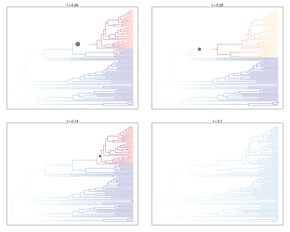
> summary(cset)
95 % credible set of rate shift configurations sampled with BAMM
Distinct shift configurations in credible set: 4
Frequency of 4 shift configurations with highest posterior probability:
rank probability cumulative Core_shifts
1 0.462 0.462 1
2 0.286 0.748 1
3 0.138 0.886 1
4 0.102 0.988 0
>
> # Accessing the raw frequency vector for the credible set:
> cset$frequency
[1] 0.462 0.286 0.138 0.102
>
> #The cumulative frequencies:
> cset$cumulative
[1] 0.462 0.748 0.886 0.988
>
> # The first element is the shift configuration with the maximum
> # a posteriori probability. We can identify all the samples from
> # posterior that show this shift configuration:
>
> cset$indices[[1]]
[1] 8 11 13 17 19 20 24 25 26 31 33 34 35 37 41 44 52 55
[19] 60 62 70 71 72 75 76 77 78 80 81 84 86 87 90 95 96 97
[37] 100 102 104 105 107 110 119 123 128 132 137 138 139 141 143 148 149 150
[55] 154 155 156 159 162 165 166 172 174 176 177 178 179 182 183 185 186 191
[73] 192 193 194 198 200 201 204 206 209 210 211 212 213 216 217 221 226 227
[91] 229 230 231 232 233 234 235 240 241 244 245 246 247 249 252 253 254 255
[109] 257 260 261 265 266 269 270 273 274 275 277 280 283 285 286 287 288 290
[127] 292 293 294 295 297 300 301 303 305 307 316 318 319 323 324 325 326 327
[145] 328 330 331 332 336 337 340 344 345 346 349 350 351 352 353 359 367 369
[163] 370 371 374 381 385 386 388 390 392 394 395 396 399 400 401 402 404 406
[181] 409 411 412 414 417 418 419 420 422 423 424 427 428 429 430 431 432 434
[199] 435 436 440 441 443 444 445 447 450 451 457 458 461 463 468 469 471 474
[217] 476 478 479 480 481 483 486 488 489 491 492 493 496 499 500
>
> # Now we can plot the credible set:
> plot(cset, plotmax=4)
Omitted 0 plots
>
>
>
>
>
> dev.off()
null device
1
>
|