Plot BAMM-estimated macroevolutionary rates on a phylogeny

Description

plot.bammdata plots a phylogenetic tree from a bammdata object and colors each branch by the estimated rate of speciation, extinction, or trait evolution. Rates are not assumed to be constant in time, and the function can plot continuously-varying rates along individual branches.

Usage

## S3 method for class 'bammdata'
plot(x, tau = 0.01, method = "phylogram", xlim = NULL,
  ylim = NULL, vtheta = 5, rbf = 0.001, show = TRUE, labels = FALSE,
  legend = FALSE, spex = "s", lwd = 1, cex = 1, pal = "RdYlBu",
  mask = integer(0), mask.color = gray(0.5), colorbreaks = NULL,
  logcolor = FALSE, breaksmethod = "linear", color.interval = NULL,
  JenksSubset = 20000, par.reset = FALSE, direction = "rightwards", ...)

Arguments

Details

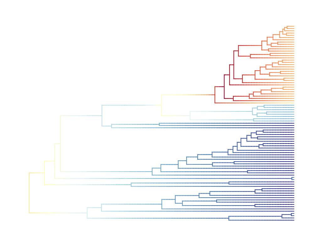
To calculate rates, each branch of the phylogeny is discretized into a number of small segments, and the mean of the marginal posterior density of the rate of speciation/extinction or trait evolution is calculated for each such segment. Rates are mapped to colors such that cool colors represent slow rates and warm colors represent fast rates. When the tree is plotted each of these small segments is plotted so that changes in rates through time and shifts in rates are visible as gradients of color. The spex argument determines the type of rate that will be calculated. spex = "s" will plot speciation rates, spex = "e" will plot extinction rates, and spex = "netdiv" will plot diversification rates (speciation - extinction). Note that if x$type = "trait" the spex argument is ignored and rates of phenotypic evolution are plotted instead. If legend = TRUE the function will plot a legend that contains the mapping of colors to numerical values.

A number of color palettes come built in with BAMMtools. Color-blind friendly options include:

• BrBG

• PiYG

• PRGn

• PuOr

• RdBu

• RdYlBu

• BuOr

• BuOrRd

• DkRdBu

• BuDkOr

• GnPu

Some color-blind unfriendly options include:

• RdYlGn

• Spectral

• temperature

• terrain

Some grayscale options include:

• grayscale

• revgray

For more information about these color palettes visit http://colorbrewer2.org and http://geography.uoregon.edu/datagraphics/color_scales.htm or use the help files of the R packages RColorBrewer and dichromat.

Additionally, any vector of valid named colors may also be used. The only restriction is that the length of this vector be greater than or equal to three (you can provide a single color, but in this case the entire tree will be assigned the same color). The colors should be ordered from cool to warm as the colors will be mapped from low rates to high rates in the order supplied (e.g. pal=c("darkgreen", "yellow2", "red")). The option pal = "temperature" uses the rich.colors function written by Arni Magnusson for the R package gplots.

Internally plot.bammdata checks whether or not rates have been calculated by looking for a component named "dtrates" in the bammdata object. If rates have not been calculated plot.bammdata calls dtRates with tau. Specifying smaller values for tau will result in smoother-looking rate changes on the tree. Note that smaller values of tau require more computation. If the colorbreaks argument is NULL a map of rates to colors is also made by calling assignColorBreaks with NCOLORS = 64. A user supplied colorbreaks argument can be passed as well. This allows one to plot parts of a tree while preserving the map of rates to colors that was made using rates for the entire tree.

If color.interval is defined, then those min and max values override the automatic detection of min and max. This might be useful if some small number of lineages have very high or very low rates, such that the map of colors is being skewed towards these extremes, resulting in other rate variation being drowned out. If specified, the color ramp will be built between these two color.interval values, and the rates outside of the color interval range will be set to the highest and lowest color.

If plot.bammdata is called repeatedly with the same bammdata object, computation can be reduced by first calling dtRates in the global environment.

Value

Returns (invisibly) a list with three components.

• coords A matrix of plot coordinates. Rows correspond to branches. Columns 1-2 are starting (x,y) coordinates of each branch and columns 3-4 are ending (x,y) coordinates of each branch. If method = "polar" a fifth column gives the angle(in radians) of each branch.

• colorbreaks A vector of percentiles used to group macroevolutionary rates into color bins.

• colordens A matrix of the kernel density estimates (column 2) of evolutionary rates (column 1) and the color (column 3) corresponding to each rate value.

Author(s)

Mike Grundler, Pascal Title

Source

http://colorbrewer2.org, http://geography.uoregon.edu/datagraphics/color_scales.htm

See Also

dtRates, addBAMMshifts, assignColorBreaks, subtreeBAMM, colorRampPalette

Examples

data(whales, events.whales)
ed <- getEventData(whales, events.whales, burnin=0.25, nsamples=500)

# The first call to plot.bammdata
# No calculations or assignments of rates have been made
plot(ed, lwd = 3, spex = "s") # calls dtRates & assignColorBreaks

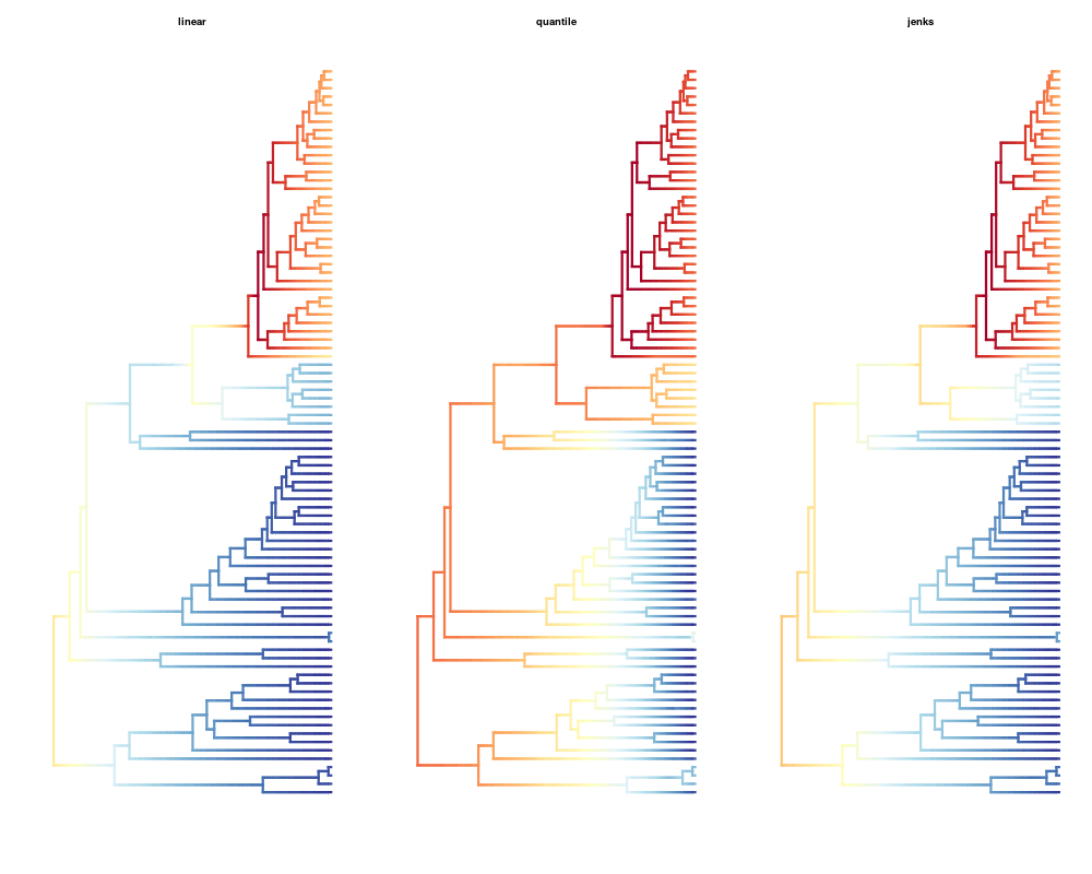
# Compare the different color breaks methods
par(mfrow=c(1,3))
plot(ed, lwd = 3, spex = "s", breaksmethod = "linear")
title(main="linear")
plot(ed, lwd = 3, spex = "s", breaksmethod = "quantile")
title(main="quantile")
plot(ed, lwd = 3, spex = "s", breaksmethod = "jenks")
title(main="jenks")

## Not run: 
# now plot.bammdata no longer calls dtRates
ed <- dtRates(ed, tau = 0.01)
xx <- plot(ed, lwd = 3, spex = "s")

# you can plot subtrees while preserving the original 
# rates to colors map by passing the colorbreaks object as an argument
sed <- subtreeBAMM(ed, node = 103)
plot(sed, lwd = 3, colorbreaks = xx$colorbreaks)
sed <- subtreeBAMM(ed, node = 140)
plot(sed, lwd = 3, colorbreaks = xx$colorbreaks)
# note how if we do not pass colorbreaks the map is 
# no longer relative to the rest of the tree and the plot is quite
# distinct from the original
plot(sed, lwd = 3)

# if you want to change the value of tau and the rates to colors map for
# the entire tree
ed <- dtRates(ed, tau = 0.002)
xx <- plot(ed, lwd = 3, spex = "s")
# now you can re-plot the subtrees using this finer tau partition
sed <- subtreeBAMM(ed, node = 103)
sed <- dtRates(sed, 0.002)
plot(sed, lwd = 3, colorbreaks = xx$colorbreaks)
sed <- subtreeBAMM(ed, node = 140)
sed <- dtRates(sed, 0.002)
plot(sed, lwd = 3, colorbreaks = xx$colorbreaks)

# multi-panel plotting and adding shifts of specific posterior samples
par(mfrow=c(2,3))
samples <- sample(1:length(ed$eventData), 6)
ed <- dtRates(ed, 0.005)
# individual plots will have a color map relative to the mean
xx <- plot(ed, show=FALSE)
for (i in 1:6) {
    ed <- dtRates(ed, 0.005, samples[i])
    plot(ed, colorbreaks=xx$colorbreaks)
    addBAMMshifts(ed,index=samples[i],method="phylogram", par.reset=FALSE)	
}
dev.off()

# color options
ed <- dtRates(ed,0.01)
plot(ed, pal="temperature",lwd=3)
plot(ed, pal="terrain",lwd=3)
plot(ed, pal=c("darkgreen","yellow2","red"),lwd=3)
plot(ed,method="polar",pal="Spectral", lwd=3)
plot(ed,method="polar",pal="RdYlBu", lwd=3)
## End(Not run)

Results

R version 3.3.1 (2016-06-21) -- "Bug in Your Hair"
Copyright (C) 2016 The R Foundation for Statistical Computing
Platform: x86_64-pc-linux-gnu (64-bit)

R is free software and comes with ABSOLUTELY NO WARRANTY.
You are welcome to redistribute it under certain conditions.
Type 'license()' or 'licence()' for distribution details.

R is a collaborative project with many contributors.
Type 'contributors()' for more information and
'citation()' on how to cite R or R packages in publications.

Type 'demo()' for some demos, 'help()' for on-line help, or
'help.start()' for an HTML browser interface to help.
Type 'q()' to quit R.

> library(BAMMtools)
Loading required package: ape
> png(filename="/home/ddbj/snapshot/RGM3/R_CC/result/BAMMtools/plot.bammdata.Rd_%03d_medium.png", width=480, height=480)
> ### Name: plot.bammdata
> ### Title: Plot 'BAMM'-estimated macroevolutionary rates on a phylogeny
> ### Aliases: plot.bammdata
> ### Keywords: graphics models
> 
> ### ** Examples
> 
> data(whales, events.whales)
> ed <- getEventData(whales, events.whales, burnin=0.25, nsamples=500)
Processing event data from data.frame

Discarded as burnin: GENERATIONS <  2495000
Analyzing  500  samples from posterior

Setting recursive sequence on tree...

Done with recursive sequence

> 
> # The first call to plot.bammdata
> # No calculations or assignments of rates have been made
> plot(ed, lwd = 3, spex = "s") # calls dtRates & assignColorBreaks
> 
> # Compare the different color breaks methods
> par(mfrow=c(1,3))
> plot(ed, lwd = 3, spex = "s", breaksmethod = "linear")
> title(main="linear")
> plot(ed, lwd = 3, spex = "s", breaksmethod = "quantile")
> title(main="quantile")
> plot(ed, lwd = 3, spex = "s", breaksmethod = "jenks")
> title(main="jenks")
> 
> ## Not run: 
> ##D # now plot.bammdata no longer calls dtRates
> ##D ed <- dtRates(ed, tau = 0.01)
> ##D xx <- plot(ed, lwd = 3, spex = "s")
> ##D 
> ##D # you can plot subtrees while preserving the original 
> ##D # rates to colors map by passing the colorbreaks object as an argument
> ##D sed <- subtreeBAMM(ed, node = 103)
> ##D plot(sed, lwd = 3, colorbreaks = xx$colorbreaks)
> ##D sed <- subtreeBAMM(ed, node = 140)
> ##D plot(sed, lwd = 3, colorbreaks = xx$colorbreaks)
> ##D # note how if we do not pass colorbreaks the map is 
> ##D # no longer relative to the rest of the tree and the plot is quite
> ##D # distinct from the original
> ##D plot(sed, lwd = 3)
> ##D 
> ##D # if you want to change the value of tau and the rates to colors map for
> ##D # the entire tree
> ##D ed <- dtRates(ed, tau = 0.002)
> ##D xx <- plot(ed, lwd = 3, spex = "s")
> ##D # now you can re-plot the subtrees using this finer tau partition
> ##D sed <- subtreeBAMM(ed, node = 103)
> ##D sed <- dtRates(sed, 0.002)
> ##D plot(sed, lwd = 3, colorbreaks = xx$colorbreaks)
> ##D sed <- subtreeBAMM(ed, node = 140)
> ##D sed <- dtRates(sed, 0.002)
> ##D plot(sed, lwd = 3, colorbreaks = xx$colorbreaks)
> ##D 
> ##D # multi-panel plotting and adding shifts of specific posterior samples
> ##D par(mfrow=c(2,3))
> ##D samples <- sample(1:length(ed$eventData), 6)
> ##D ed <- dtRates(ed, 0.005)
> ##D # individual plots will have a color map relative to the mean
> ##D xx <- plot(ed, show=FALSE)
> ##D for (i in 1:6) {
> ##D     ed <- dtRates(ed, 0.005, samples[i])
> ##D     plot(ed, colorbreaks=xx$colorbreaks)
> ##D     addBAMMshifts(ed,index=samples[i],method="phylogram", par.reset=FALSE)	
> ##D }
> ##D dev.off()
> ##D 
> ##D # color options
> ##D ed <- dtRates(ed,0.01)
> ##D plot(ed, pal="temperature",lwd=3)
> ##D plot(ed, pal="terrain",lwd=3)
> ##D plot(ed, pal=c("darkgreen","yellow2","red"),lwd=3)
> ##D plot(ed,method="polar",pal="Spectral", lwd=3)
> ##D plot(ed,method="polar",pal="RdYlBu", lwd=3)
> ## End(Not run)
> 
> 
> 
> 
> 
> dev.off()
null device 
          1 
>