Bayesian Composition Estimator

Description

This function estimates taxonomic compositions of algal communities based on biomarker field data. More precisely, it estimates the probability distributions of a sample composition based on an input ratio matrix, A that contains prior estimates of biomarker ratios in different taxa, and an input data matrix, B, containing biomarker ratios measured in field samples.

Probability distributions are estimated based on an adaptive metropolis MCMC method, function modMCMC from package FME.

Usage

bce1(A, B, Wa=NULL, Wb=NULL,
       jmpType="default", jmpA=.1,jmpX=.1, jmpCovar=NULL,
       initX=NULL, initA=NULL, priorA="normal", minA=NULL, maxA=NULL, 
       var0=NULL, wvar0=1e-6, Xratios=TRUE, verbose=TRUE, ...)

Arguments

Details

The function bce1 searches probability distributions for all elements of a taxonomical composition matrix X and a ratio matrix A for which:

A%*%X ~= B

It does this by returning niter samples for A and X, organized in three-dimensional arrays. The input data matrix B and ratio matrix A should be in the following formats, with the relative concentrations per biomarker organized in columns:

data matrix B:

and ratio matrix A:

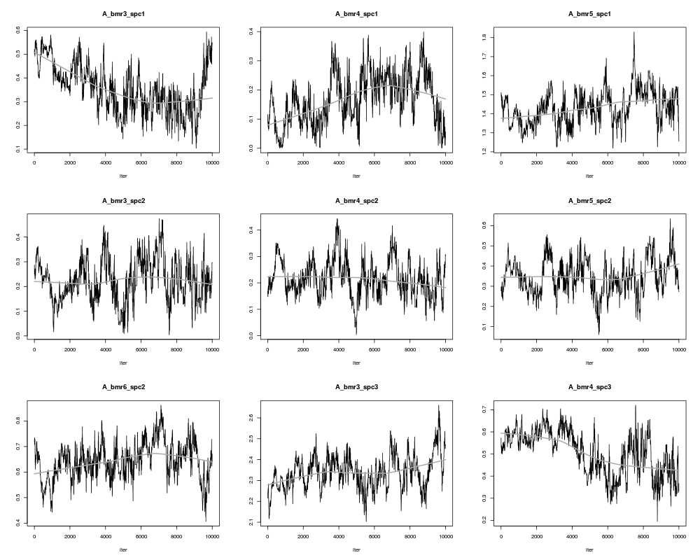
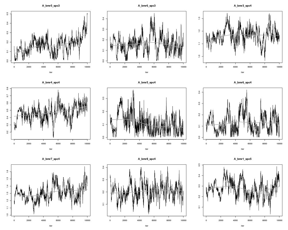
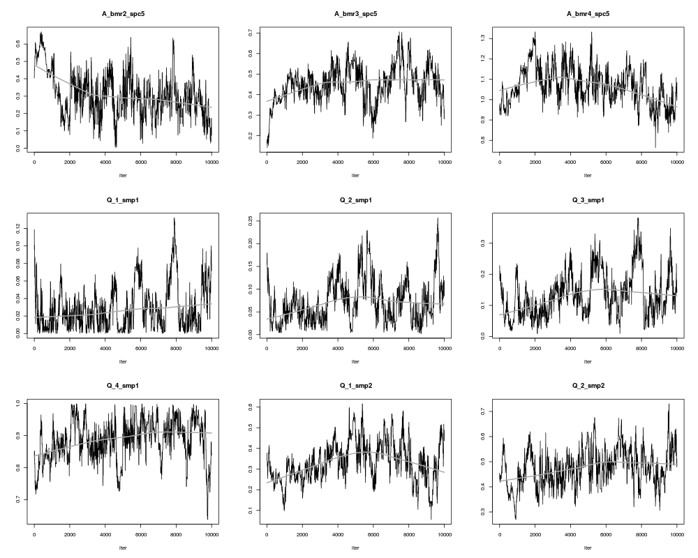
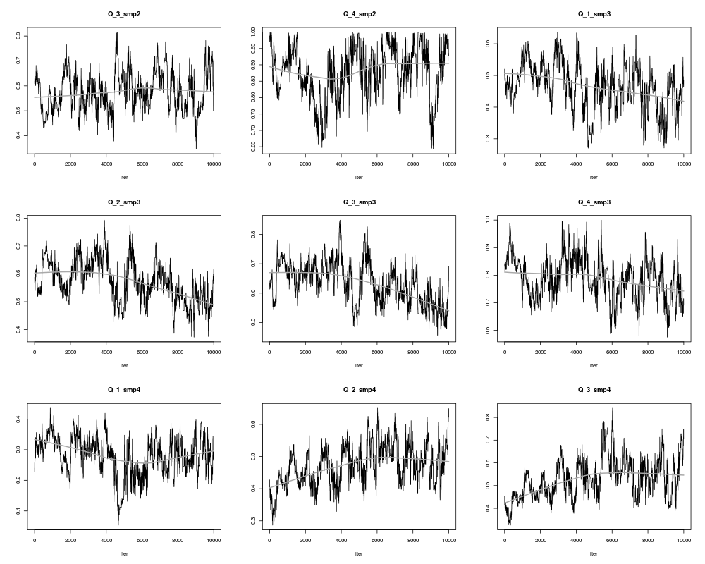
Value

An object of class bce and _modMCMC_ (returned by the function modMCMC). This object has methods for the generic functions 'summary', 'plot', 'pairs'- see ?modMCMC. It is distinguished from other modMCMC objects by 3 extra attributes that allow to extract matrices A and X from the mcmc result: "dim_A" (dimensions of A), "A_not_null" (which elements of A are not zero and thus included in the mcmc) and Xratios (whether X was rescaled, yes or no).

Note

Producing sensible output:

Markov Chain Monte Carlo simulations are not as straightforward as one might wish; several preliminary runs might be necessary to determine the desired number of iterations, burn-in length and jump length. For all estimated values of Rat and X, their trace (evolution of the values over all iterations) has to display random behaviour; no obvious trends should appear. A few parameters can be tuned to obtain such behaviour:

• jump length The jump length determines how big the jumps are for each step in the random walk. A longer jump length will make you jump around faster in the parameter space, but acceptance of new points can get very low. Smaller jump lengths increase the acceptance rate, but the algorithm will move too slowly, and a lot more runs will be needed to scan the whole parameter space. A good way to find a good jump length, is look at the number of points accepted. If the output is saved under the name MCMC, you can find the number of accepted points under MCMC$naccepted. It is also given if you run the model with verbose=TRUE (default). This value should be somewhere between 5% and 40%. For long runs, 5 % can be acceptable, for short runs, you will prefer a higher acceptance in order to have enough different points. 20% accepted is usually a good number. Do some preliminary runs with niter=1000-10000 and tune the jump length parameters jmpRat and jmpX. You can set different jump lengths for each column of the ratio matrix, or 1 jump length for the whole ratio matrix, and 1 jump length for the composition matrix. Decreasing the jump lengths will generally increase the acceptance rate and vice versa. Also the mixing rate (the speed with which accepted points change their values) will be influenced. You want this mixing rate to be as high as possible, whilst maintaining enough accepted points.

• burninlength The program uses the solution of lsei using the original ratio matrix as starting values for the MCMC. This might in some cases be far from the optimal solution, and the MCMC algorithm will start with moving towards this optimal solution. This is called a burn-in. When there is a slow mixing rate, this can take a considerable number of cycles. As it can influence the averages and standard deviations, you might want to remove it from the mcmc objects. By defining a burnin length, the first 'burninlength' cycles will not be written to the output. Look at some plots to determine if you need to specify a burnin length.

• niter the number of iterations: start with 10000 runs or less; check the output and estimate how many runs you will need to get a random pattern in the output.

Author(s)

Karel Van den Meersche <k.vdmeersche@nioo.knaw.nl>, Karline Soetaert <k.soetaert@nioo.knaw.nl>.

References

Van den Meersche, K., K. Soetaert and J.J. Middelburg (2008) A Bayesian compositional estimator for microbial taxonomy based on biomarkers, Limnology and Oceanography Methods 6, 190-199

See Also

summary.bce, plot.bce, export.bce, pairs.bce

Examples

##====================================

# example using bceInput data
# !!! should be weighted to correspond better to example of BCE!!!
A <- t(bceInput$Rat)
B <- t(bceInput$Dat)


result <- bce1(A,B,niter=1000)

## the number of accepted runs is zero;
## try different starting values

result <- bce1(A,B,niter=1000,initX=matrix(1/ncol(A),ncol(A),ncol(B)))

## number of accepted runs is still low;
## smaller jumps

result <- bce1(A,B,niter=1000,initX=matrix(1/ncol(A),ncol(A),ncol(B)),jmpA=.01,jmpX=.01)
Sum <-summary(result)

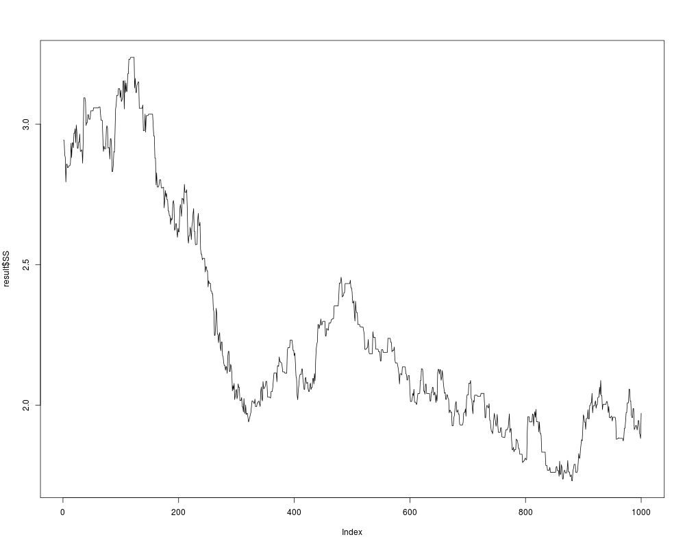
## did the algorithm converge?
plot(result$SS,type="l")
## no


## more runs, using the output of previous run as input.
result <- bce1(A,B,niter=1e4,jmpA=.01,jmpX=.01,updatecov=1e3,
               initX=Sum$lastX,initA=Sum$lastA,
               jmpCovar=Sum$covar*2.4^2/ncol(result$pars),
               )
Sum <-summary(result)

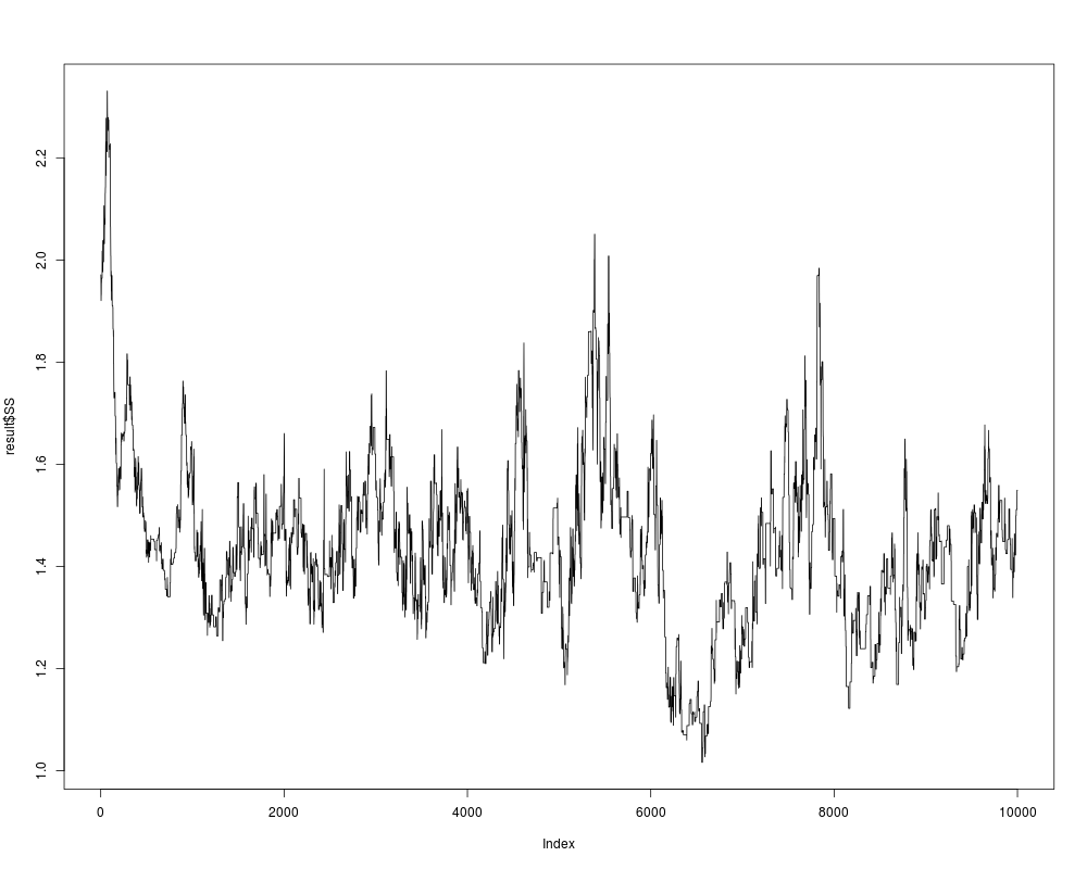
## we inspect the output:
plot(result$SS,type="l")
plot(result,ask=TRUE)
## looks already pretty good; to get a better result, repeat one more
## time with a  longer run. Uncomment the following paragraph and run.
## go get some coffee, this might take a while (~30s).

## result <- bce1(A,B,niter=1e5,jmpA=.01,jmpX=.01,updatecov=1e3,
##                outputlength=1e3,burninlength=.35e5,
##                initX=Sum$lastX,initA=Sum$lastA,
##                jmpCovar=Sum$covar*2.4^2/ncol(result$pars),
##                )
## Sum <-summary(result)
## plot(result$SS,type="l")
## plot(result,ask=TRUE)

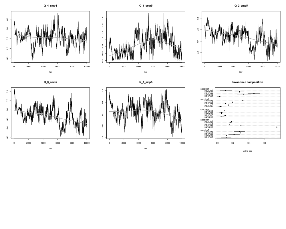
# show results as mean with ranges
print(Sum$meanX)

# plot estimated means and ranges (lbX=lower, ubX=upper bound)
xlim <- range(c(Sum$lbX,Sum$ubX))

# first the mean
dotchart(x=t(Sum$meanX),xlim=xlim,                                                          
         main="Taxonomic composition",
         sub="using bce",pch=16)

# then ranges
nr <- nrow(Sum$meanX)
nc <- ncol(Sum$meanX)

for (i in 1:nr) 
  {ip <-(nr-i)*(nc+2)+1
   cc <- ip : (ip+nc-1)
   segments(t(Sum$lbX[i,]),cc,t(Sum$ubX[i,]),cc)
  }

Results

R version 3.3.1 (2016-06-21) -- "Bug in Your Hair"
Copyright (C) 2016 The R Foundation for Statistical Computing
Platform: x86_64-pc-linux-gnu (64-bit)

R is free software and comes with ABSOLUTELY NO WARRANTY.
You are welcome to redistribute it under certain conditions.
Type 'license()' or 'licence()' for distribution details.

R is a collaborative project with many contributors.
Type 'contributors()' for more information and
'citation()' on how to cite R or R packages in publications.

Type 'demo()' for some demos, 'help()' for on-line help, or
'help.start()' for an HTML browser interface to help.
Type 'q()' to quit R.

> library(BCE)
Loading required package: FME
Loading required package: deSolve

Attaching package: 'deSolve'

The following object is masked from 'package:graphics':

    matplot

Loading required package: rootSolve
Loading required package: coda
Loading required package: limSolve
Loading required package: Matrix
> png(filename="/home/ddbj/snapshot/RGM3/R_CC/result/BCE/bce1.Rd_%03d_medium.png", width=480, height=480)
> ### Name: bce1
> ### Title: Bayesian Composition Estimator
> ### Aliases: bce1 bce
> ### Keywords: models
> 
> ### ** Examples
> 
> ##====================================
> 
> # example using bceInput data
> # !!! should be weighted to correspond better to example of BCE!!!
> A <- t(bceInput$Rat)
> B <- t(bceInput$Dat)
> 
> 
> result <- bce1(A,B,niter=1000)
number of accepted runs: 0 out of 1000 (0%) 
> 
> ## the number of accepted runs is zero;
> ## try different starting values
> 
> result <- bce1(A,B,niter=1000,initX=matrix(1/ncol(A),ncol(A),ncol(B)))
number of accepted runs: 3 out of 1000 (0.3%) 
> 
> ## number of accepted runs is still low;
> ## smaller jumps
> 
> result <- bce1(A,B,niter=1000,initX=matrix(1/ncol(A),ncol(A),ncol(B)),jmpA=.01,jmpX=.01)
number of accepted runs: 599 out of 1000 (59.9%) 
> Sum <-summary(result)
> 
> ## did the algorithm converge?
> plot(result$SS,type="l")
> ## no
> 
> 
> ## more runs, using the output of previous run as input.
> result <- bce1(A,B,niter=1e4,jmpA=.01,jmpX=.01,updatecov=1e3,
+                initX=Sum$lastX,initA=Sum$lastA,
+                jmpCovar=Sum$covar*2.4^2/ncol(result$pars),
+                )
number of accepted runs: 2231 out of 10000 (22.31%) 
> Sum <-summary(result)
> 
> ## we inspect the output:
> plot(result$SS,type="l")
> plot(result,ask=TRUE)
> ## looks already pretty good; to get a better result, repeat one more
> ## time with a  longer run. Uncomment the following paragraph and run.
> ## go get some coffee, this might take a while (~30s).
> 
> ## result <- bce1(A,B,niter=1e5,jmpA=.01,jmpX=.01,updatecov=1e3,
> ##                outputlength=1e3,burninlength=.35e5,
> ##                initX=Sum$lastX,initA=Sum$lastA,
> ##                jmpCovar=Sum$covar*2.4^2/ncol(result$pars),
> ##                )
> ## Sum <-summary(result)
> ## plot(result$SS,type="l")
> ## plot(result,ask=TRUE)
> 
> # show results as mean with ranges
> print(Sum$meanX)
            sample1    sample2    sample3    sample4    sample5
species1 0.05961017 0.26185310 0.31148917 0.26198854 0.11634095
species2 0.07009629 0.26325358 0.14119779 0.21569245 0.14203054
species3 0.06221225 0.08024785 0.07674516 0.07383608 0.06040147
species4 0.71671509 0.20937915 0.21846790 0.12876959 0.27164753
species5 0.09136619 0.18526632 0.25209999 0.31971333 0.40957951
> 
> # plot estimated means and ranges (lbX=lower, ubX=upper bound)
> xlim <- range(c(Sum$lbX,Sum$ubX))
> 
> # first the mean
> dotchart(x=t(Sum$meanX),xlim=xlim,                                                          
+          main="Taxonomic composition",
+          sub="using bce",pch=16)
> 
> # then ranges
> nr <- nrow(Sum$meanX)
> nc <- ncol(Sum$meanX)
> 
> for (i in 1:nr) 
+   {ip <-(nr-i)*(nc+2)+1
+    cc <- ip : (ip+nc-1)
+    segments(t(Sum$lbX[i,]),cc,t(Sum$ubX[i,]),cc)
+   }
> 
> 
> 
> 
> 
> 
> dev.off()
null device 
          1 
>