R Graphical Manual

Browse All

Last data update: 2014.03.03

R: Bayesian Cost-Effectiveness Analysis

bcea	R Documentation

Bayesian Cost-Effectiveness Analysis

Description

Cost-effectiveness analysis based on the results of a simulation model for a variable of clinical benefits (e) and of costs (c). Produces results to be post-processed to give the health economic analysis. The output is stored in an object of the class "bcea"

Usage

bcea(e, c, ref = 1, interventions = NULL, Kmax = 50000, 
     wtp = NULL, plot = FALSE)

## Default S3 method:
bcea(e, c, ref = 1, interventions = NULL, Kmax = 50000, 
     wtp = NULL, plot = FALSE)

Arguments

`e`	An object containing `nsim` simulations for the variable of clinical effectiveness for each intervention being considered. In general it is a matrix with `nsim` rows and `nint` columns.
`c`	An object containing `nsim` simulations for the variable of cost for each intervention being considered. In general it is a matrix with `nsim` rows and `nint` columns.
`ref`	Defines which intervention (columns of `e` or `c`) is considered to be the reference strategy. The default value `ref=1` means that the intervention associated with the first column of `e` or `c` is the reference and the one(s) associated with the other column(s) is(are) the comparators.
`interventions`	Defines the labels to be associated with each intervention. By default and if `NULL`, assigns labels in the form "Intervention1", ... , "Intervention T".
`Kmax`	Maximum value of the willingness to pay to be considered. Default value is `k=50000`. The willingness to pay is then approximated on a discrete grid in the interval `[0,Kmax]`. The grid is equal to `wtp` if the parameter is given, or composed of `501` elements if `wtp=NULL` (the default).
`wtp`	A(n optional) vector wtp including the values of the willingness to pay grid. If not specified then BCEA will construct a grid of 501 values from 0 to Kmax. This option is useful when performing intensive computations (eg for the EVPPI).
`plot`	A logical value indicating whether the function should produce the summary plot or not.

Value

An object of the class "bcea" containing the following elements

`n.sim`	Number of simulations produced by the Bayesian model
`n.comparators`	Number of interventions being analysed
`n.comparisons`	Number of possible pairwise comparisons
`delta.e`	For each possible comparison, the differential in the effectiveness measure
`delta.c`	For each possible comparison, the differential in the cost measure
`ICER`	The value of the Incremental Cost-Effectiveness Ratio
`Kmax`	The maximum value assumed for the willingness to pay threshold
`k`	The vector of values for the grid approximation of the willingness to pay
`ceac`	The value for the Cost-Effectiveness Acceptability Curve, as a function of the willingness to pay
`ib`	The distribution of the Incremental Benefit, for a given willingness to pay
`eib`	The value for the Expected Incremental Benefit, as a function of the willingness to pay
`kstar`	The grid approximation of the break even point(s)
`best`	A vector containing the numeric label of the intervention that is the most cost-effective for each value of the willingness to pay in the selected grid approximation
`U`	An array including the value of the expected utility for each simulation from the Bayesian model, for each value of the grid approximation of the willingness to pay and for each intervention being considered
`vi`	An array including the value of information for each simulation from the Bayesian model and for each value of the grid approximation of the willingness to pay
`Ustar`	An array including the maximum "known-distribution" utility for each simulation from the Bayesian model and for each value of the grid approximation of the willingness to pay
`ol`	An array including the opportunity loss for each simulation from the Bayesian model and for each value of the grid approximation of the willingness to pay
`evi`	The vector of values for the Expected Value of Information, as a function of the willingness to pay
`interventions`	A vector of labels for all the interventions considered
`ref`	The numeric index associated with the intervention used as reference in the analysis
`comp`	The numeric index(es) associated with the intervention(s) used as comparator(s) in the analysis
`step`	The step used to form the grid approximation to the willingness to pay
`e`	The `e` matrix used to generate the object (see Arguments)
`c`	The `c` matrix used to generate the object (see Arguments)

Author(s)

Gianluca Baio, Andrea Berardi

References

Baio, G., Dawid, A. P. (2011). Probabilistic Sensitivity Analysis in Health Economics. Statistical Methods in Medical Research doi:10.1177/0962280211419832.

Baio G. (2012). Bayesian Methods in Health Economics. CRC/Chapman Hall, London

Examples

# See Baio G., Dawid A.P. (2011) for a detailed description of the 
# Bayesian model and economic problem
#
# Load the processed results of the MCMC simulation model
data(Vaccine)
# 
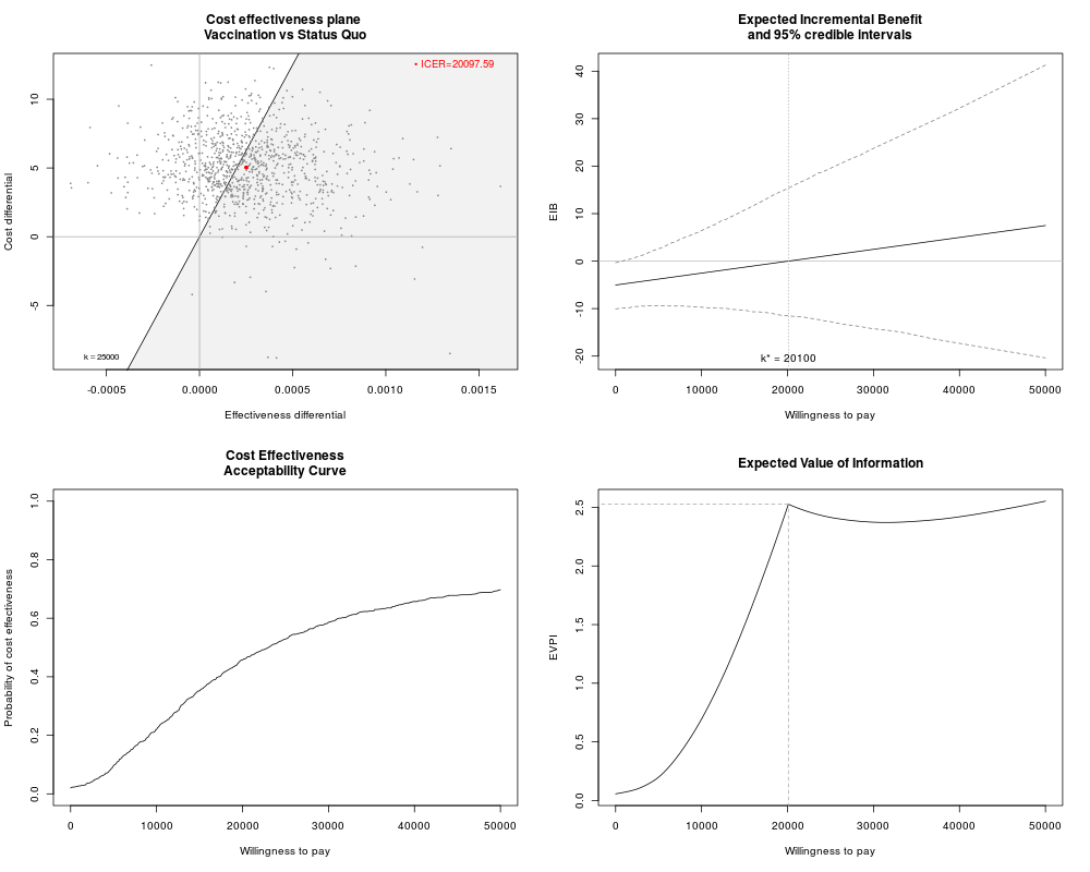
# Runs the health economic evaluation using BCEA
m <- bcea(e=e,c=c,          # defines the variables of 
                            #  effectiveness and cost
      ref=2,                # selects the 2nd row of (e,c) 
                            #  as containing the reference intervention
      interventions=treats, # defines the labels to be associated 
                            #  with each intervention
      Kmax=50000,           # maximum value possible for the willingness 
                            #  to pay threshold; implies that k is chosen 
                            #  in a grid from the interval (0,Kmax)
      plot=TRUE          # plots the results
)
#
# Creates a summary table
summary(m,      # uses the results of the economic evalaution 
                #  (a "bcea" object)
      wtp=25000	# selects the particular value for k 
)


#
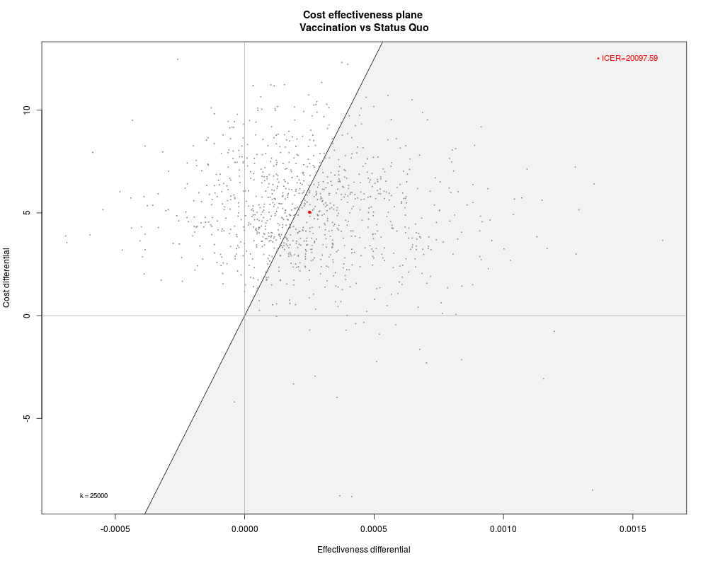
# Plots the cost-effectiveness plane using base graphics
ceplane.plot(m,      # plots the Cost-Effectiveness plane
      comparison=1,  # if more than 2 interventions, selects the
                     #  pairwise comparison 
      wtp=25000,     # selects the relevant willingness to pay 
                     #  (default: 25,000) 
      graph="base"   # selects base graphics (default)
)
#
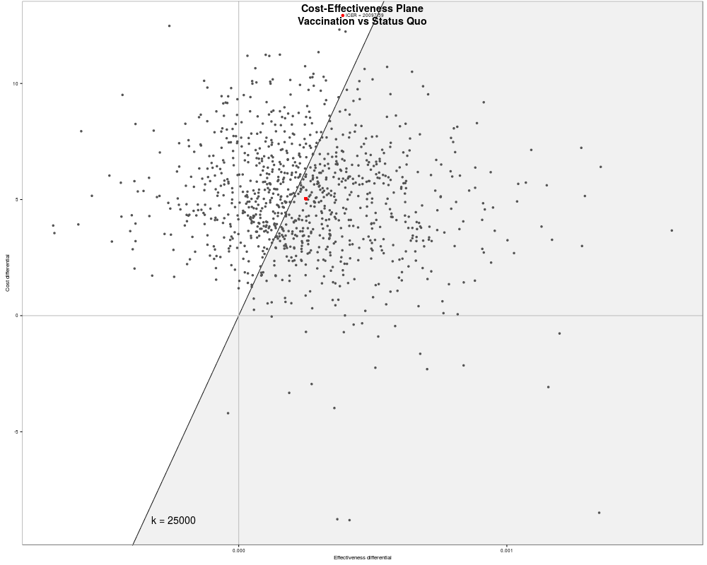
# Plots the cost-effectiveness plane using ggplot2
if(requireNamespace("ggplot2")){
ceplane.plot(m,      # plots the Cost-Effectiveness plane
      comparison=1,  # if more than 2 interventions, selects the
                     #  pairwise comparison 
      wtp=25000,     # selects the relevant willingness to pay 
                     #  (default: 25,000) 
      graph="ggplot2"# selects ggplot2 as the graphical engine
)
#
# Some more options
ceplane.plot(m,
      graph="ggplot2",
      pos="top",
      size=5,
      ICER.size=1.5,
      label.pos=FALSE,
      opt.theme=ggplot2::theme(text=ggplot2::element_text(size=8))
)
}
#
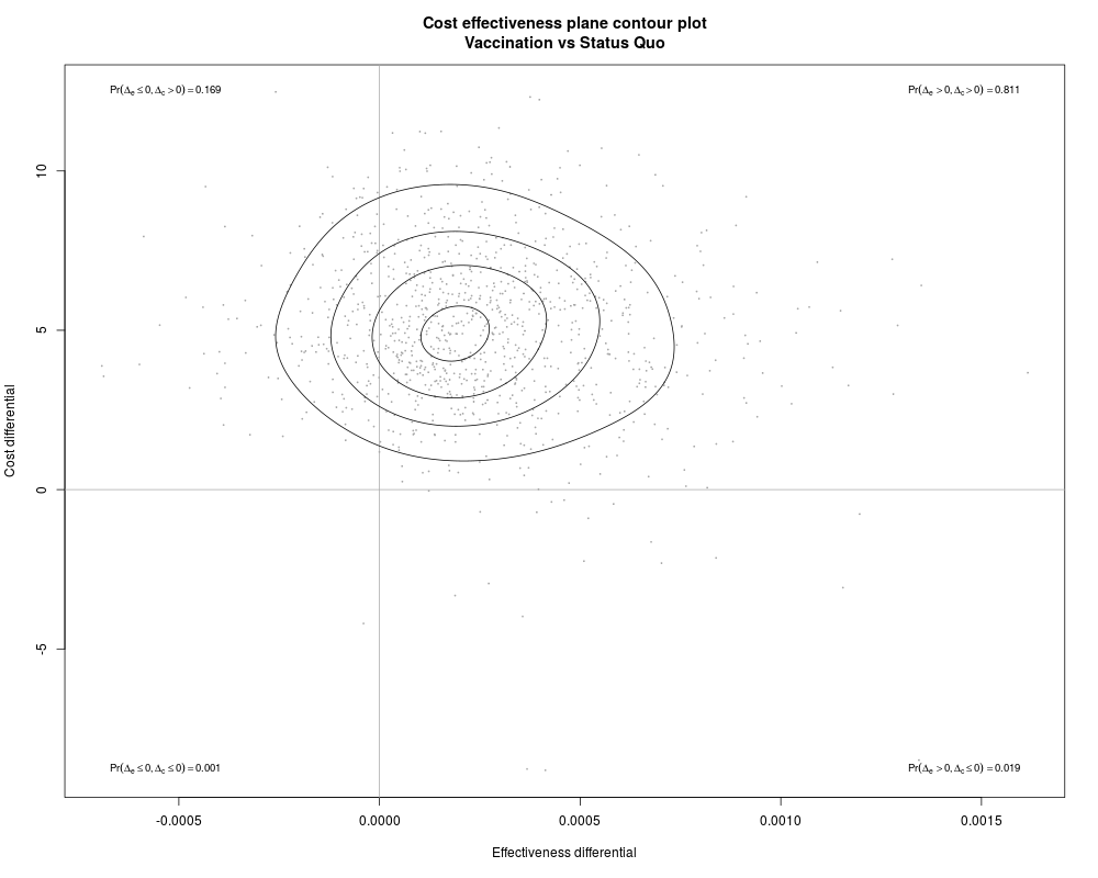
# Plots the contour and scatterplot of the bivariate 
# distribution of (Delta_e,Delta_c)
contour(m,          # uses the results of the economic evalaution 
                    #  (a "bcea" object)
      comparison=1, # if more than 2 interventions, selects the 
                    #  pairwise comparison 
      nlevels=4,    # selects the number of levels to be 
                    #  plotted (default=4)
      levels=NULL,  # specifies the actual levels to be plotted 
                    #  (default=NULL, so that R will decide)
      scale=0.5,    # scales the bandwiths for both x- and 
                    #  y-axis (default=0.5)
      graph="base"  # uses base graphics to produce the plot
)
#
# Plots the contour and scatterplot of the bivariate 
#   distribution of (Delta_e,Delta_c)
contour2(m,       # uses the results of the economic evalaution 
                  #  (a "bcea" object)
      wtp=25000,  # selects the willingness-to-pay threshold
      xl=NULL,    # assumes default values
      yl=NULL     # assumes default values
)
#
# Using ggplot2
if(requireNamespace("ggplot2")){
contour2(m,           # uses the results of the economic evalaution 
                      #  (a "bcea" object)
      graph="ggplot2",# selects the graphical engine
      wtp=25000,      # selects the willingness-to-pay threshold
      xl=NULL,        # assumes default values
      yl=NULL,        # assumes default values
      label.pos=FALSE # alternative position for the wtp label
)
}
#
# Plots the Expected Incremental Benefit for the "bcea" object m
eib.plot(m)
#
# Plots the distribution of the Incremental Benefit
ib.plot(m,        # uses the results of the economic evalaution 
                  #  (a "bcea" object)
    comparison=1, # if more than 2 interventions, selects the 
                  #  pairwise comparison 
    wtp=25000,    # selects the relevant willingness 
                  #  to pay (default: 25,000)
    graph="base"  # uses base graphics
)
#
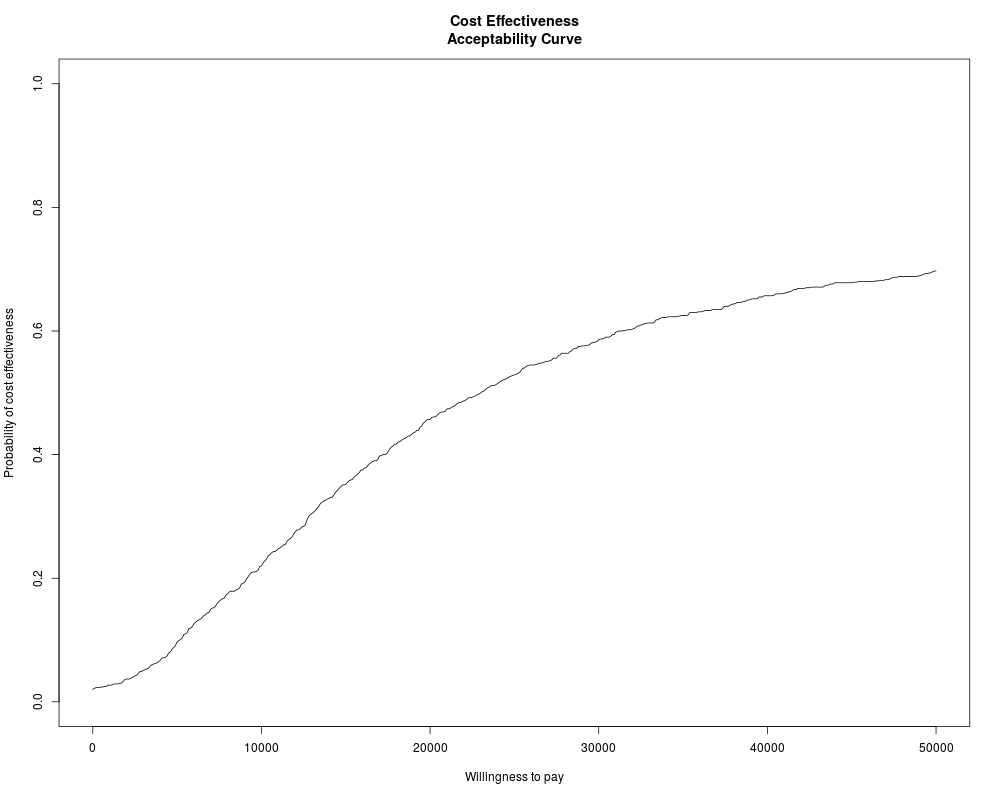
# Produces a plot of the CEAC against a grid of values for the 
# willingness to pay threshold
ceac.plot(m)
#
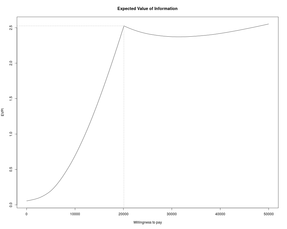
# Plots the Expected Value of Information for the "bcea" object m
evi.plot(m)
#

Results


R version 3.3.1 (2016-06-21) -- "Bug in Your Hair"
Copyright (C) 2016 The R Foundation for Statistical Computing
Platform: x86_64-pc-linux-gnu (64-bit)

R is free software and comes with ABSOLUTELY NO WARRANTY.
You are welcome to redistribute it under certain conditions.
Type 'license()' or 'licence()' for distribution details.

R is a collaborative project with many contributors.
Type 'contributors()' for more information and
'citation()' on how to cite R or R packages in publications.

Type 'demo()' for some demos, 'help()' for on-line help, or
'help.start()' for an HTML browser interface to help.
Type 'q()' to quit R.

> library(BCEA)
> png(filename="/home/ddbj/snapshot/RGM3/R_CC/result/BCEA/bcea.Rd_%03d_medium.png", width=480, height=480)
> ### Name: bcea
> ### Title: Bayesian Cost-Effectiveness Analysis
> ### Aliases: bcea bcea.default CEanalysis
> ### Keywords: Health economic evaluation
> 
> ### ** Examples
> 
> # See Baio G., Dawid A.P. (2011) for a detailed description of the 
> # Bayesian model and economic problem
> #
> # Load the processed results of the MCMC simulation model
> data(Vaccine)
> # 
> # Runs the health economic evaluation using BCEA
> m <- bcea(e=e,c=c,          # defines the variables of 
+                             #  effectiveness and cost
+       ref=2,                # selects the 2nd row of (e,c) 
+                             #  as containing the reference intervention
+       interventions=treats, # defines the labels to be associated 
+                             #  with each intervention
+       Kmax=50000,           # maximum value possible for the willingness 
+                             #  to pay threshold; implies that k is chosen 
+                             #  in a grid from the interval (0,Kmax)
+       plot=TRUE          # plots the results
+ )
> #
> # Creates a summary table
> summary(m,      # uses the results of the economic evalaution 
+                 #  (a "bcea" object)
+       wtp=25000	# selects the particular value for k 
+ )

Cost-effectiveness analysis summary 

Reference intervention:  Vaccination
Comparator intervention: Status Quo

Optimal decision: choose Status Quo for k<20100 and Vaccination for k>=20100


Analysis for willingness to pay parameter k = 25000

            Expected utility
Status Quo           -36.054
Vaccination          -34.826

                             EIB  CEAC  ICER
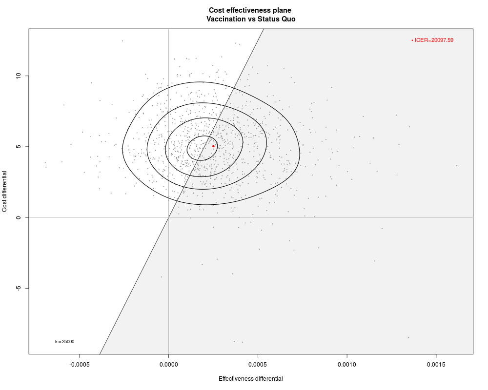
Vaccination vs Status Quo 1.2284 0.529 20098

Optimal intervention (max expected utility) for k=25000: Vaccination
           
EVPI 2.4145
> 
> ## No test: 
> #
> # Plots the cost-effectiveness plane using base graphics
> ceplane.plot(m,      # plots the Cost-Effectiveness plane
+       comparison=1,  # if more than 2 interventions, selects the
+                      #  pairwise comparison 
+       wtp=25000,     # selects the relevant willingness to pay 
+                      #  (default: 25,000) 
+       graph="base"   # selects base graphics (default)
+ )
> #
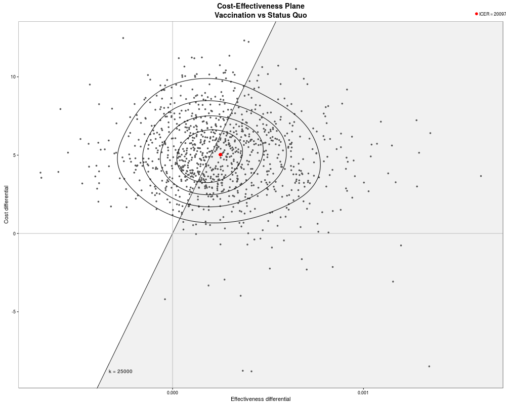
> # Plots the cost-effectiveness plane using ggplot2
> if(requireNamespace("ggplot2")){
+ ceplane.plot(m,      # plots the Cost-Effectiveness plane
+       comparison=1,  # if more than 2 interventions, selects the
+                      #  pairwise comparison 
+       wtp=25000,     # selects the relevant willingness to pay 
+                      #  (default: 25,000) 
+       graph="ggplot2"# selects ggplot2 as the graphical engine
+ )
+ #
+ # Some more options
+ ceplane.plot(m,
+       graph="ggplot2",
+       pos="top",
+       size=5,
+       ICER.size=1.5,
+       label.pos=FALSE,
+       opt.theme=ggplot2::theme(text=ggplot2::element_text(size=8))
+ )
+ }
Loading required namespace: ggplot2
> #
> # Plots the contour and scatterplot of the bivariate 
> # distribution of (Delta_e,Delta_c)
> contour(m,          # uses the results of the economic evalaution 
+                     #  (a "bcea" object)
+       comparison=1, # if more than 2 interventions, selects the 
+                     #  pairwise comparison 
+       nlevels=4,    # selects the number of levels to be 
+                     #  plotted (default=4)
+       levels=NULL,  # specifies the actual levels to be plotted 
+                     #  (default=NULL, so that R will decide)
+       scale=0.5,    # scales the bandwiths for both x- and 
+                     #  y-axis (default=0.5)
+       graph="base"  # uses base graphics to produce the plot
+ )
Loading required namespace: MASS
> #
> # Plots the contour and scatterplot of the bivariate 
> #   distribution of (Delta_e,Delta_c)
> contour2(m,       # uses the results of the economic evalaution 
+                   #  (a "bcea" object)
+       wtp=25000,  # selects the willingness-to-pay threshold
+       xl=NULL,    # assumes default values
+       yl=NULL     # assumes default values
+ )
The first available comparison will be selected. To plot multiple comparisons together please use the ggplot2 version. Please see ?contour2 for additional details.
> #
> # Using ggplot2
> if(requireNamespace("ggplot2")){
+ contour2(m,           # uses the results of the economic evalaution 
+                       #  (a "bcea" object)
+       graph="ggplot2",# selects the graphical engine
+       wtp=25000,      # selects the willingness-to-pay threshold
+       xl=NULL,        # assumes default values
+       yl=NULL,        # assumes default values
+       label.pos=FALSE # alternative position for the wtp label
+ )
+ }
> #
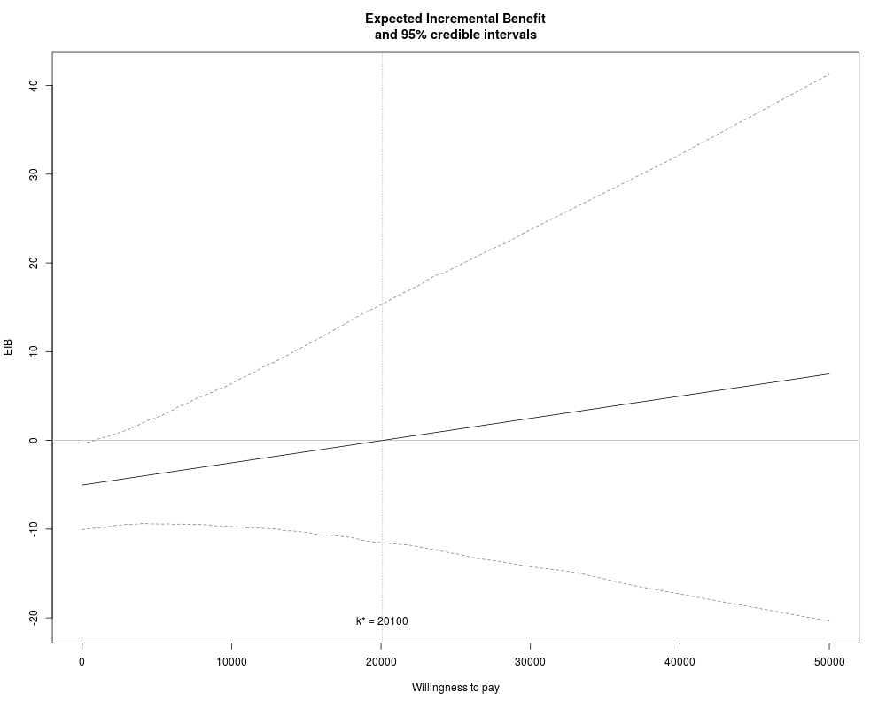
> # Plots the Expected Incremental Benefit for the "bcea" object m
> eib.plot(m)
> #
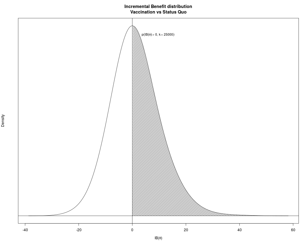
> # Plots the distribution of the Incremental Benefit
> ib.plot(m,        # uses the results of the economic evalaution 
+                   #  (a "bcea" object)
+     comparison=1, # if more than 2 interventions, selects the 
+                   #  pairwise comparison 
+     wtp=25000,    # selects the relevant willingness 
+                   #  to pay (default: 25,000)
+     graph="base"  # uses base graphics
+ )
> #
> # Produces a plot of the CEAC against a grid of values for the 
> # willingness to pay threshold
> ceac.plot(m)
> #
> # Plots the Expected Value of Information for the "bcea" object m
> evi.plot(m)
> #
> ## End(No test)
> 
> 
> 
> 
> 
> dev.off()
null device 
          1 
>