Cost-Effectiveness Efficiency Frontier (CEAF) plot

Description

Produces a plot of the Cost-Effectiveness Efficiency Frontier (CEEF)

Usage

ceef.plot(he, comparators = NULL, pos = c(1, 1), 
start.from.origins = TRUE, threshold = NULL, flip = FALSE, 
dominance = TRUE, relative = FALSE, print.summary = TRUE, 
graph = c("base", "ggplot2"), ...)

Arguments

Details

The bcea objects did not include the generating e and c matrices in BCEA versions <2.1-0. This function is not compatible with objects created with previous versions. The matrices can be appended to bcea objects obtained using previous versions, making sure that the class of the object remains unaltered.

The argument print.summary allows for printing a brief summary of the efficiency frontier, with default to TRUE. Two tables are plotted, one for the interventions included in the frontier and one for the dominated interventions. The average costs and clinical benefits are included for each intervention. The frontier table includes the slope for the increase in the frontier and the non-frontier table displays the dominance type of each dominated intervention. Please note that the slopes are defined as the increment in the costs for a unit increment in the benefits even if flip = TRUE for consistency with the ICER definition. The angle of increase is in radians and depends on the definition of the axes, i.e. on the value given to the flip argument.

If the argument relative is set to TRUE, the graph will not display the absolute measures of costs and benefits. Instead the axes will represent differential costs and benefits compared to the reference intervention (indexed by ref in the bcea function).

Value

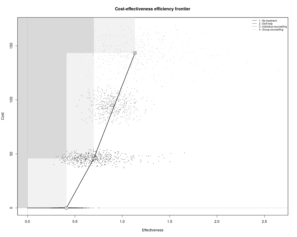
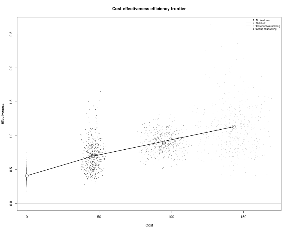
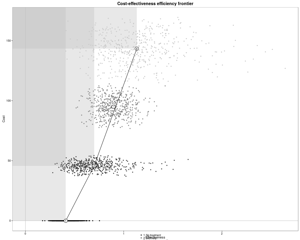
The function produces a plot of the cost-effectiveness efficiency frontier. The dots show the simulated values for the intervention-specific distributions of the effectiveness and costs. The circles indicate the average of each bivariate distribution, with the numbers referring to each included intervention. The numbers inside the circles are black if the intervention is included in the frontier and grey otherwise. If the option dominance is set to TRUE, the dominance regions are plotted, indicating the areas of dominance. Interventions in the areas between the dominance region and the frontier are in a situation of extended dominance.

Author(s)

Andrea Berardi, Gianluca Baio

References

Baio G. (2012). Bayesian Methods in Health Economics. CRC/Chapman Hall, London.

IQWIG (2009). General methods for the Assessment of the Relation of Benefits to Cost, Version 1.0. IQWIG, November 2009.

See Also

bcea

Examples

### create the bcea object m for the smoking cessation example
data(Smoking)
m <- bcea(e,c,ref=4,Kmax=500,interventions=treats)
### produce the plot
ceef.plot(m,graph="base")

### tweak the options
ceef.plot(m,flip=TRUE,dominance=FALSE,start.from.origins=FALSE,
          print.summary=FALSE,graph="base")
### or use ggplot2 instead
if(require(ggplot2)){
ceef.plot(m,dominance=TRUE,start.from.origins=FALSE,pos=TRUE,
          print.summary=FALSE,graph="ggplot2")
}

Results

R version 3.3.1 (2016-06-21) -- "Bug in Your Hair"
Copyright (C) 2016 The R Foundation for Statistical Computing
Platform: x86_64-pc-linux-gnu (64-bit)

R is free software and comes with ABSOLUTELY NO WARRANTY.
You are welcome to redistribute it under certain conditions.
Type 'license()' or 'licence()' for distribution details.

R is a collaborative project with many contributors.
Type 'contributors()' for more information and
'citation()' on how to cite R or R packages in publications.

Type 'demo()' for some demos, 'help()' for on-line help, or
'help.start()' for an HTML browser interface to help.
Type 'q()' to quit R.

> library(BCEA)
> png(filename="/home/ddbj/snapshot/RGM3/R_CC/result/BCEA/ceef.plot.Rd_%03d_medium.png", width=480, height=480)
> ### Name: ceef.plot
> ### Title: Cost-Effectiveness Efficiency Frontier (CEAF) plot
> ### Aliases: ceef.plot
> ### Keywords: Health economic evaluation Multiple comparisons
> 
> ### ** Examples
> 
> ### create the bcea object m for the smoking cessation example
> data(Smoking)
> m <- bcea(e,c,ref=4,Kmax=500,interventions=treats)
> ### produce the plot
> ceef.plot(m,graph="base")

Cost-effectiveness efficiency frontier summary 

Interventions on the efficiency frontier:
                  Effectiveness   Costs Increase slope Increase angle
No treatment            0.41051   0.000           0.00         0.0000
Self-help               0.69875  45.733         158.66         1.5645
Group counselling       1.13303 143.301         224.67         1.5663

Interventions not on the efficiency frontier:
                       Effectiveness  Costs     Dominance type
Individual counselling       0.89536 94.919 Extended dominance
> ## No test: 
> ### tweak the options
> ceef.plot(m,flip=TRUE,dominance=FALSE,start.from.origins=FALSE,
+           print.summary=FALSE,graph="base")
> ### or use ggplot2 instead
> if(require(ggplot2)){
+ ceef.plot(m,dominance=TRUE,start.from.origins=FALSE,pos=TRUE,
+           print.summary=FALSE,graph="ggplot2")
+ }
Loading required package: ggplot2
> ## End(No test)
> 
> 
> 
> 
> 
> dev.off()
null device 
          1 
>