R Graphical Manual

Browse All

Last data update: 2014.03.03

R: Cost-effectiveness plane plot

ceplane.plot

R Documentation

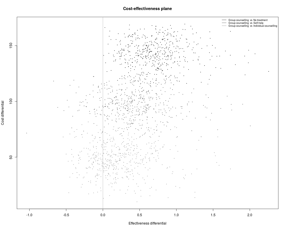
Cost-effectiveness plane plot

Description

Produces a scatter plot of the cost-effectiveness plane, together with the sustainability area, as a function of the selected willingness to pay threshold

Usage

ceplane.plot(he, comparison = NULL, wtp = 25000, pos=c(1,1), 
size=NULL, graph=c("base","ggplot2"), 
xlim=NULL, ylim=NULL, ...)

Arguments

`he`	A `bcea` object containing the results of the Bayesian modelling and the economic evaluation.
`comparison`	Selects the comparator, in case of more than two interventions being analysed. Default as `NULL` plots all the comparisons together. Any subset of the possible comparisons can be selected (e.g., `comparison=c(1,3)` or `comparison=2`).
`wtp`	The value of the willingness to pay parameter. Not used iff `graph="base"` for multiple comparisons.
`pos`	Parameter to set the position of the legend; for a single comparison plot, the ICER legend position. Can be given in form of a string `(bottom\|top)(right\|left)` for base graphics and `bottom\|top\|left\|right` for ggplot2. It can be a two-elements vector, which specifies the relative position on the x and y axis respectively, or alternatively it can be in form of a logical variable, with `FALSE` indicating to use the default position and `TRUE` to place it on the bottom of the plot. Default value is `c(1,1)`, that is the topright corner inside the plot area.
`size`	Value (in millimetres) of the size of the willingness to pay label. Used only if `graph="ggplot2"`, otherwise is ignored with a message.
`graph`	A string used to select the graphical engine to use for plotting. Should (partial-)match the two options `"base"` or `"ggplot2"`. Default value is `"base"`.
`xlim`	The range of the plot along the x-axis. If NULL (default) it is determined by the range of the simulated values for `delta.e`
`ylim`	The range of the plot along the y-axis. If NULL (default) it is determined by the range of the simulated values for `delta.c`
`...`	If `graph="ggplot2"` and a named theme object is supplied, it will be added to the ggplot object. In addition, if `graph="ggplot2"`, `ICER.size` can be used to resize the red dot representing the ICER (i.e. showing them if multiple comparisons are selected), and `label.pos=FALSE` will place the willingness to pay label in a different position at the bottom of the graph.

Value

ceplane

A ggplot object containing the plot. Returned only if graph="ggplot2".

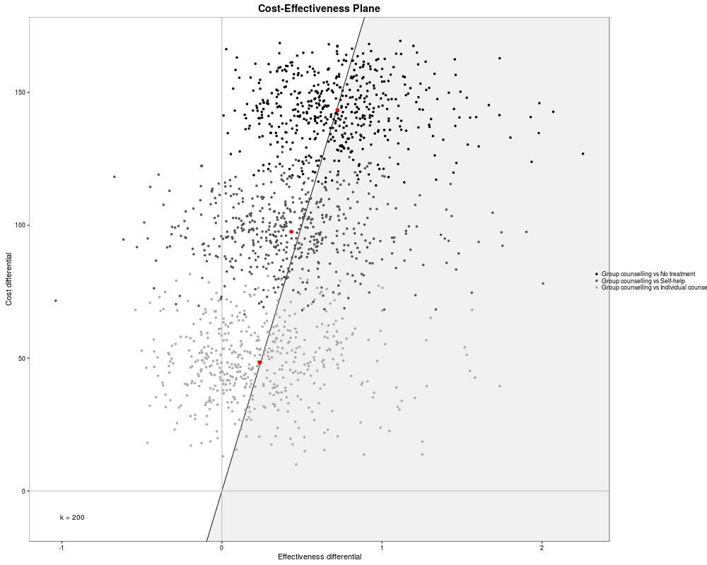
The function produces a plot of the cost-effectiveness plane. Grey dots show the simulated values for the joint distribution of the effectiveness and cost differentials. The larger red dot shows the ICER and the grey area identifies the sustainability area, i.e. the part of the plan for which the simulated values are below the willingness to pay threshold. The proportion of points in the sustainability area effectively represents the CEAC for a given value of the willingness to pay. If the comparators are more than 2 and no pairwise comparison is specified, all scatterplots are graphed using different colors.

Author(s)

Gianluca Baio, Andrea Berardi

References

Baio, G., Dawid, A. P. (2011). Probabilistic Sensitivity Analysis in Health Economics. Statistical Methods in Medical Research doi:10.1177/0962280211419832.

Baio G. (2012). Bayesian Methods in Health Economics. CRC/Chapman Hall, London

Examples

### create the bcea object m for the smoking cessation example
data(Smoking)
m <- bcea(e,c,ref=4,Kmax=500,interventions=treats)
### produce the plot
ceplane.plot(m,wtp=200,graph="base")
### select only one comparator
ceplane.plot(m,wtp=200,graph="base",comparator=3)
### or use ggplot2 instead
if(requireNamespace("ggplot2")){
ceplane.plot(m,wtp=200,pos="right",ICER.size=2,graph="ggplot2")
}

Results


R version 3.3.1 (2016-06-21) -- "Bug in Your Hair"
Copyright (C) 2016 The R Foundation for Statistical Computing
Platform: x86_64-pc-linux-gnu (64-bit)

R is free software and comes with ABSOLUTELY NO WARRANTY.
You are welcome to redistribute it under certain conditions.
Type 'license()' or 'licence()' for distribution details.

R is a collaborative project with many contributors.
Type 'contributors()' for more information and
'citation()' on how to cite R or R packages in publications.

Type 'demo()' for some demos, 'help()' for on-line help, or
'help.start()' for an HTML browser interface to help.
Type 'q()' to quit R.

> library(BCEA)
> png(filename="/home/ddbj/snapshot/RGM3/R_CC/result/BCEA/ceplane.plot.Rd_%03d_medium.png", width=480, height=480)
> ### Name: ceplane.plot
> ### Title: Cost-effectiveness plane plot
> ### Aliases: ceplane.plot
> ### Keywords: Health economic evaluation Cost Effectiveness Plane
> 
> ### ** Examples
> 
> ### create the bcea object m for the smoking cessation example
> data(Smoking)
> m <- bcea(e,c,ref=4,Kmax=500,interventions=treats)
> ### produce the plot
> ceplane.plot(m,wtp=200,graph="base")
> ### select only one comparator
> ceplane.plot(m,wtp=200,graph="base",comparator=3)
> ### or use ggplot2 instead
> if(requireNamespace("ggplot2")){
+ ceplane.plot(m,wtp=200,pos="right",ICER.size=2,graph="ggplot2")
+ }
Loading required namespace: ggplot2
> 
> 
> 
> 
> 
> dev.off()
null device 
          1 
>