R Graphical Manual

Browse All

Last data update: 2014.03.03

R: Specialised contour plot for objects in the class "bcea"

contour2

R Documentation

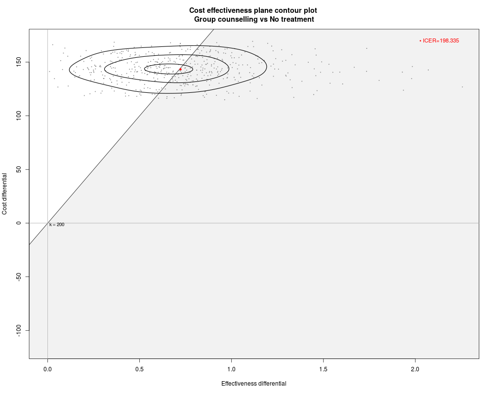
Specialised contour plot for objects in the class "bcea"

Description

Produces a scatterplot of the cost-effectiveness plane, with a contour-plot of the bivariate density of the differentials of cost (y-axis) and effectiveness (x-axis). Also adds the sustainability area (i.e. below the selected value of the willingness-to-pay threshold).

Usage

contour2(he, wtp=25000, xlim=NULL, ylim=NULL, comparison=NULL, 
         graph=c("base","ggplot2"),...)

Arguments

`he`	A "bcea" object containing the results of the Bayesian modelling and the economic evaluation
`wtp`	The selected value of the willingness-to-pay. Default is `25000`.
`xlim`	Limits on the x-axis (default=`NULL`, so that R will select appropriate limits).
`ylim`	Limits on the y-axis (default=`NULL`, so that R will select appropriate limits).
`comparison`	The comparison being plotted. Default to `NULL` chooses the first comparison if `graph="base"`. If `graph="ggplot2"` the default value will choose all the possible comparisons. Any subset of the possible comparisons can be selected (e.g., `comparison=c(1,3)`).
`graph`	A string used to select the graphical engine to use for plotting. Should (partial-)match the two options `"base"` or `"ggplot2"`. Default value is `"base"`.
`...`	Arguments to be passed to `ceplane.plot`. See the relative manual page for more details.

Value

contour

A ggplot item containing the requested plot. Returned only if graph="ggplot2".

Plots the cost-effectiveness plane with a scatterplot of all the simulated values from the (posterior) bivariate distribution of (Delta_e,Delta_c), the differentials of effectiveness and costs; superimposes a contour of the distribution and prints the value of the ICER, together with the sustainability area.

Author(s)

Gianluca Baio, Andrea Berardi

References

Baio, G., Dawid, A. P. (2011). Probabilistic Sensitivity Analysis in Health Economics. Statistical Methods in Medical Research doi:10.1177/0962280211419832.

Baio G. (2012). Bayesian Methods in Health Economics. CRC/Chapman Hall, London

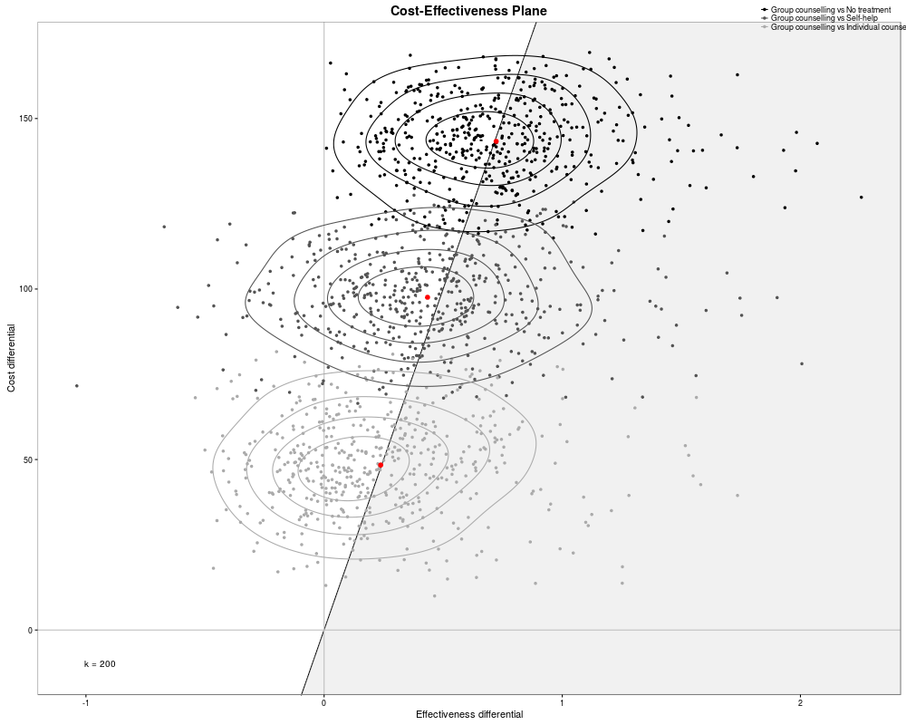
Examples

### create the bcea object m for the smoking cessation example
data(Smoking)
m=bcea(e,c,ref=4,interventions=treats,Kmax=500)
### produce the plot
contour2(m,wtp=200,graph="base")

### or use ggplot2 to plot multiple comparisons
contour2(m,wtp=200,ICER.size=2,graph="ggplot2")

Results


R version 3.3.1 (2016-06-21) -- "Bug in Your Hair"
Copyright (C) 2016 The R Foundation for Statistical Computing
Platform: x86_64-pc-linux-gnu (64-bit)

R is free software and comes with ABSOLUTELY NO WARRANTY.
You are welcome to redistribute it under certain conditions.
Type 'license()' or 'licence()' for distribution details.

R is a collaborative project with many contributors.
Type 'contributors()' for more information and
'citation()' on how to cite R or R packages in publications.

Type 'demo()' for some demos, 'help()' for on-line help, or
'help.start()' for an HTML browser interface to help.
Type 'q()' to quit R.

> library(BCEA)
> png(filename="/home/ddbj/snapshot/RGM3/R_CC/result/BCEA/contour2.Rd_%03d_medium.png", width=480, height=480)
> ### Name: contour2
> ### Title: Specialised contour plot for objects in the class "bcea"
> ### Aliases: contour2
> ### Keywords: Health economic evaluation Bayesian model
> 
> ### ** Examples
> 
> ### create the bcea object m for the smoking cessation example
> data(Smoking)
> m=bcea(e,c,ref=4,interventions=treats,Kmax=500)
> ### produce the plot
> contour2(m,wtp=200,graph="base")
The first available comparison will be selected. To plot multiple comparisons together please use the ggplot2 version. Please see ?contour2 for additional details.
Loading required namespace: MASS
> ## No test: 
> ### or use ggplot2 to plot multiple comparisons
> contour2(m,wtp=200,ICER.size=2,graph="ggplot2")
> ## End(No test)
> 
> 
> 
> 
> 
> dev.off()
null device 
          1 
>