Summary plot of the health economic analysis when risk aversion is included

Description

Plots the EIB and the EVPI when risk aversion is included in the utility function

Usage

## S3 method for class 'CEriskav'
plot(x, pos=c(0,1), graph=c("base","ggplot2"), ...)

Arguments

Value

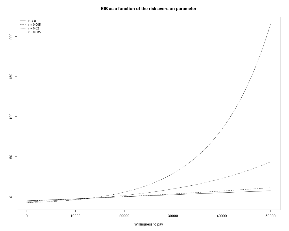
The function produces two plots for the risk aversion analysis. The first one is the EIB as a function of the discrete grid approximation of the willingness parameter for each of the possible values of the risk aversion parameter, r. The second one is a similar plot for the EVPI.

Author(s)

Gianluca Baio, Andrea Berardi

References

Baio, G., Dawid, A. P. (2011). Probabilistic Sensitivity Analysis in Health Economics. Statistical Methods in Medical Research doi:10.1177/0962280211419832.

Baio G. (2012). Bayesian Methods in Health Economics. CRC/Chapman Hall, London

See Also

bcea, CEriskav

Examples

# See Baio G., Dawid A.P. (2011) for a detailed description of the 
# Bayesian model and economic problem
#
# Load the processed results of the MCMC simulation model
data(Vaccine)
# 
# Runs the health economic evaluation using BCEA
m <- bcea(e=e,c=c,          # defines the variables of 
                            #  effectiveness and cost
      ref=2,                # selects the 2nd row of (e,c) 
                            #  as containing the reference intervention
      interventions=treats, # defines the labels to be associated 
                            #  with each intervention
      Kmax=50000,           # maximum value possible for the willingness 
                            #  to pay threshold; implies that k is chosen 
                            #  in a grid from the interval (0,Kmax)
      plot=FALSE            # inhibits graphical output
)
#
# Define the vector of values for the risk aversion parameter, r, eg:
r <- c(0.000000000001,0.005,0.020,0.035) 
#
# Run the cost-effectiveness analysis accounting for risk aversion

cr <- CEriskav(m,     # uses the results of the economic evalaution 
                      #  (a "bcea" object)
        r=r,          # defines the vector of values for the risk 
                      #  aversion parameter
        comparison=1  # if more than 2 interventions, selects the 
                      #  pairwise comparison 
)

#
# Now produce the plots

plot(cr # uses the results of the risk aversion 
        #  analysis (a "CEriskav" object)
)

### Alternative options, using ggplot2

plot(cr,
  graph="ggplot2",
  plot="ask"          # plot option can be specified as
                      #  "dev.new" (default), "x11" or "ask"
  )

Results

R version 3.3.1 (2016-06-21) -- "Bug in Your Hair"
Copyright (C) 2016 The R Foundation for Statistical Computing
Platform: x86_64-pc-linux-gnu (64-bit)

R is free software and comes with ABSOLUTELY NO WARRANTY.
You are welcome to redistribute it under certain conditions.
Type 'license()' or 'licence()' for distribution details.

R is a collaborative project with many contributors.
Type 'contributors()' for more information and
'citation()' on how to cite R or R packages in publications.

Type 'demo()' for some demos, 'help()' for on-line help, or
'help.start()' for an HTML browser interface to help.
Type 'q()' to quit R.

> library(BCEA)
> png(filename="/home/ddbj/snapshot/RGM3/R_CC/result/BCEA/plot.CEriskav.Rd_%03d_medium.png", width=480, height=480)
> ### Name: plot.CEriskav
> ### Title: Summary plot of the health economic analysis when risk aversion
> ###   is included
> ### Aliases: plot.CEriskav
> ### Keywords: Health economic evaluation Risk aversion
> 
> ### ** Examples
> 
> # See Baio G., Dawid A.P. (2011) for a detailed description of the 
> # Bayesian model and economic problem
> #
> # Load the processed results of the MCMC simulation model
> data(Vaccine)
> # 
> # Runs the health economic evaluation using BCEA
> m <- bcea(e=e,c=c,          # defines the variables of 
+                             #  effectiveness and cost
+       ref=2,                # selects the 2nd row of (e,c) 
+                             #  as containing the reference intervention
+       interventions=treats, # defines the labels to be associated 
+                             #  with each intervention
+       Kmax=50000,           # maximum value possible for the willingness 
+                             #  to pay threshold; implies that k is chosen 
+                             #  in a grid from the interval (0,Kmax)
+       plot=FALSE            # inhibits graphical output
+ )
> #
> # Define the vector of values for the risk aversion parameter, r, eg:
> r <- c(0.000000000001,0.005,0.020,0.035) 
> #
> # Run the cost-effectiveness analysis accounting for risk aversion
> ## No test: 
> cr <- CEriskav(m,     # uses the results of the economic evalaution 
+                       #  (a "bcea" object)
+         r=r,          # defines the vector of values for the risk 
+                       #  aversion parameter
+         comparison=1  # if more than 2 interventions, selects the 
+                       #  pairwise comparison 
+ )
> ## End(No test)
> #
> # Now produce the plots
> ## No test: 
> plot(cr # uses the results of the risk aversion 
+         #  analysis (a "CEriskav" object)
+ )
dev.new(): using pdf(file="Rplots14.pdf")
> ## End(No test)
> ### Alternative options, using ggplot2
> ## No test: 
> plot(cr,
+   graph="ggplot2",
+   plot="ask"          # plot option can be specified as
+                       #  "dev.new" (default), "x11" or "ask"
+   )
> ## End(No test)
> 
> 
> 
> 
> 
> dev.off()
png 
  2 
>