R Graphical Manual

Browse All

Last data update: 2014.03.03

R: Summary plot of the health economic analysis

plot.bcea

R Documentation

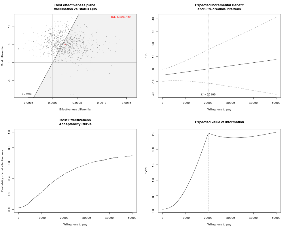
Summary plot of the health economic analysis

Description

Plots in a single graph the Cost-Effectiveness plane, the Expected Incremental Benefit, the CEAC and the EVPI

Usage

## S3 method for class 'bcea'
plot(x, comparison=NULL, wtp=25000, pos=FALSE, 
graph=c("base","ggplot2"), ...)

Arguments

`x`	A `bcea` object containing the results of the Bayesian modelling and the economic evaluation.
`comparison`	Selects the comparator, in case of more than two interventions being analysed. The value is passed to `ceplane.plot`, `eib.plot` and `ceac.plot`.
`wtp`	The value of the willingness to pay parameter. It is passed to `ceplane.plot`.
`pos`	Parameter to set the position of the legend. Can be given in form of a string, a single logical value, or a two-element vector with the respective relative positions on the x and y axis. Default as `FALSE` sets the legend position to the default one for each plot (see the details section), while `TRUE` puts it on the bottom of each plot. Changes will affect all the individual plots.
`graph`	A string used to select the graphical engine to use for plotting. Should (partial-)match the two options `"base"` or `"ggplot2"`. Default value is `"base"`.
`...`	Arguments to be passed to the methods `ceplane.plot` and `eib.plot`. Please see the manual pages for the individual functions. Arguments like `size`, `ICER.size` and `plot.cri` can be supplied to the functions in this way. In addition if `graph="ggplot2"` and the arguments are named theme objects they will be added to each plot.

Details

The default position of the legend for the cost-effectiveness plane (produced by ceplane.plot) is set to c(1,1.025) overriding its default for pos=FALSE, since multiple ggplot2 plots are rendered in a slightly different way than single plots.

For more information see the documentation of each individual plot function.

Value

The function produces a plot with four graphical summaries of the health economic evaluation.

Author(s)

Gianluca Baio, Andrea Berardi

References

Baio, G., Dawid, A. P. (2011). Probabilistic Sensitivity Analysis in Health Economics. Statistical Methods in Medical Research doi:10.1177/0962280211419832.

Baio G. (2012). Bayesian Methods in Health Economics. CRC/Chapman Hall, London

Examples

# See Baio G., Dawid A.P. (2011) for a detailed description of the 
# Bayesian model and economic problem
#
# Load the processed results of the MCMC simulation model
data(Vaccine)
# 
# Runs the health economic evaluation using BCEA
m <- bcea(e=e,c=c,          # defines the variables of 
                            #  effectiveness and cost
      ref=2,                # selects the 2nd row of (e,c) 
                            #  as containing the reference intervention
      interventions=treats, # defines the labels to be associated 
                            #  with each intervention
      Kmax=50000,           # maximum value possible for the willingness 
                            #  to pay threshold; implies that k is chosen 
                            #  in a grid from the interval (0,Kmax)
      plot=FALSE            # does not produce graphical outputs
)
#
# Plots the summary plots for the "bcea" object m using base graphics
plot(m,graph="base")

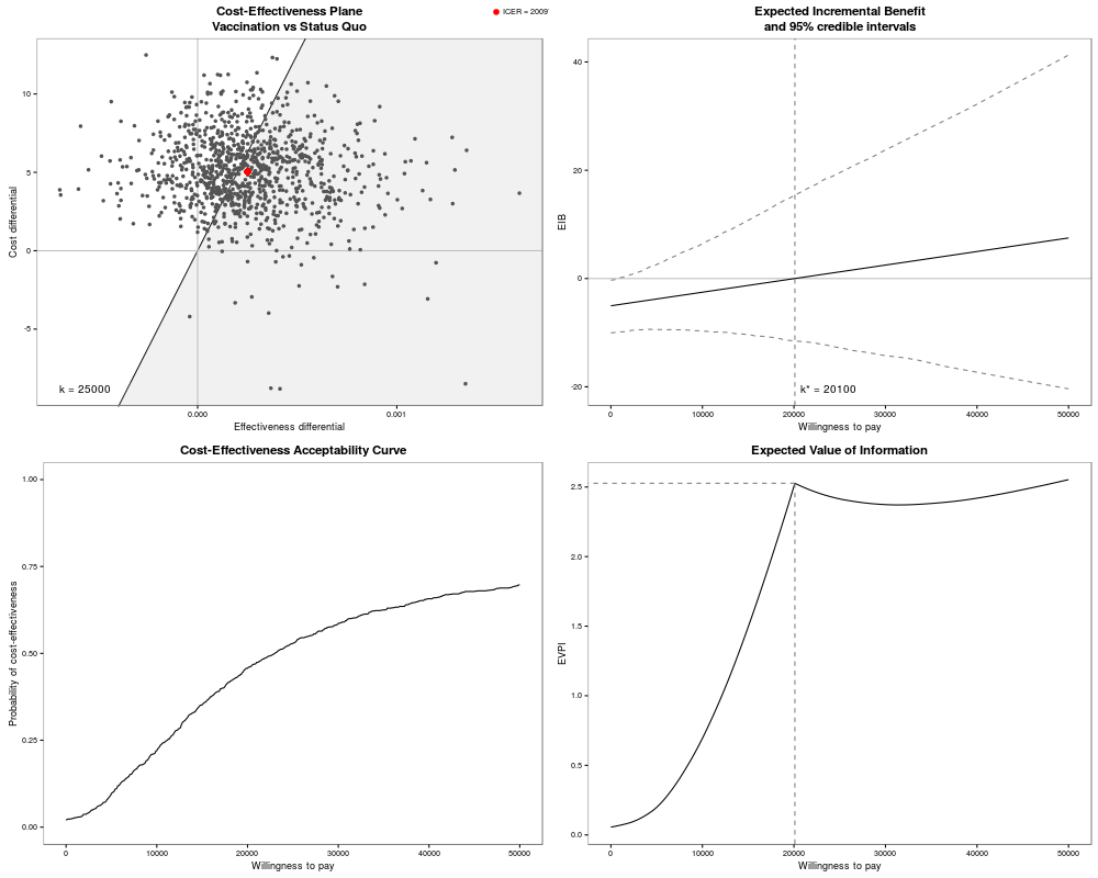
# Plots the same summary plots using ggplot2
if(require(ggplot2)){
plot(m,graph="ggplot2")

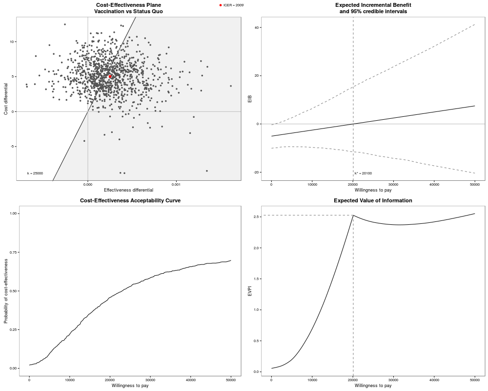
##### Example of a customized plot.bcea with ggplot2
plot(m,
  graph="ggplot2",                                      # use ggplot2
  theme=theme(plot.title=element_text(size=rel(1.25))), # theme elements must have a name
  ICER.size=1.5,                                        # hidden option in ceplane.plot
  size=rel(2.5)                                         # modifies the size of k= labels
)                                                       #  in ceplane.plot and eib.plot
}

Results


R version 3.3.1 (2016-06-21) -- "Bug in Your Hair"
Copyright (C) 2016 The R Foundation for Statistical Computing
Platform: x86_64-pc-linux-gnu (64-bit)

R is free software and comes with ABSOLUTELY NO WARRANTY.
You are welcome to redistribute it under certain conditions.
Type 'license()' or 'licence()' for distribution details.

R is a collaborative project with many contributors.
Type 'contributors()' for more information and
'citation()' on how to cite R or R packages in publications.

Type 'demo()' for some demos, 'help()' for on-line help, or
'help.start()' for an HTML browser interface to help.
Type 'q()' to quit R.

> library(BCEA)
> png(filename="/home/ddbj/snapshot/RGM3/R_CC/result/BCEA/plot.bcea.Rd_%03d_medium.png", width=480, height=480)
> ### Name: plot.bcea
> ### Title: Summary plot of the health economic analysis
> ### Aliases: plot.bcea
> ### Keywords: Health economic evaluation
> 
> ### ** Examples
> 
> # See Baio G., Dawid A.P. (2011) for a detailed description of the 
> # Bayesian model and economic problem
> #
> # Load the processed results of the MCMC simulation model
> data(Vaccine)
> # 
> # Runs the health economic evaluation using BCEA
> m <- bcea(e=e,c=c,          # defines the variables of 
+                             #  effectiveness and cost
+       ref=2,                # selects the 2nd row of (e,c) 
+                             #  as containing the reference intervention
+       interventions=treats, # defines the labels to be associated 
+                             #  with each intervention
+       Kmax=50000,           # maximum value possible for the willingness 
+                             #  to pay threshold; implies that k is chosen 
+                             #  in a grid from the interval (0,Kmax)
+       plot=FALSE            # does not produce graphical outputs
+ )
> #
> # Plots the summary plots for the "bcea" object m using base graphics
> plot(m,graph="base")
> 
> # Plots the same summary plots using ggplot2
> if(require(ggplot2)){
+ plot(m,graph="ggplot2")
+ 
+ ##### Example of a customized plot.bcea with ggplot2
+ plot(m,
+   graph="ggplot2",                                      # use ggplot2
+   theme=theme(plot.title=element_text(size=rel(1.25))), # theme elements must have a name
+   ICER.size=1.5,                                        # hidden option in ceplane.plot
+   size=rel(2.5)                                         # modifies the size of k= labels
+ )                                                       #  in ceplane.plot and eib.plot
+ }
Loading required package: ggplot2
> 
> 
> 
> 
> 
> dev.off()
null device 
          1 
>