A named list including values for the variables e0 (measure of effectiveness for the
subjects in treatment arm t=0), e1 (effectiveness for the subjects in t=1), c0
(individual costs in t=0), c1 (individual costs in t=1), H.psi and H.zeta (vectors of
fixed hyperparameters for the prior in the positive cost groups. If only one value is
passed as argument, then BCEs0 assumes that this is to be used for both treatments being
considered). Additional optional elements are X0 (a matrix of covariates for t=0) and
X1 (a matrix of covariates for t=1) that can be used to estimate the selection model for null costs
dist.c
A text string defining the selected distribution for the costs. Available options are
Gamma ("gamma"), log-Normal ("logn") and Normal ("norm")
dist.e
A text string defining the selected distribution for the measure of effectiveness.
Available options are Beta ("beta"), Gamma ("gamma"), Bernoulli ("bern") and Normal
("norm")
w
A parameter used to characterise the mean of the degenerate distribution for the
structural zeros (default = 0.000001)
W
A parameter used to characterise the standard deviaiton of the degenerate distribution
for the structural zeros (default = 0.000001)
n.iter
Number of iterations to be run in JAGS (default = 10000)
n.burnin
Number of iterations to be used as burn-in for the MCMC procedure (default = 5000)
n.chains
Number of Markov chains to be run (default = 2)
robust
A string indicating whether a robust model should be chosen for the patter model. If
TRUE (default), then the regression coefficients are modelled using a Cauchy(0,2.5)
distribution. If FALSE, then a vague Normal prior is used
model.file
A string with the name of the txt file to which the JAGS code is saved. Default is
model.txt.
Value
An object containing the following elements
mod
A "rjags" objects with the results of the MCMC simulations run using JAGS
params
A vector including the parameters being monitored
dataJags
A list contaning the data needed to run the MCMC simulations
inits
A function used to initialise the random nodes in the model
Author(s)
Gianluca Baio
References
Baio G. (2013). Bayesian models for cost-effectiveness analysis in the presence of
structural zero costs. http://arxiv.org/pdf/1307.5243v1.pdf
Examples
data(acupuncture)
m <- bces0(data,dist.c="gamma",dist.e="beta",n.iter=1000,n.burnin=500,n.chains=2)
print(m)
plot(m)
Results
R version 3.3.1 (2016-06-21) -- "Bug in Your Hair"
Copyright (C) 2016 The R Foundation for Statistical Computing
Platform: x86_64-pc-linux-gnu (64-bit)
R is free software and comes with ABSOLUTELY NO WARRANTY.
You are welcome to redistribute it under certain conditions.
Type 'license()' or 'licence()' for distribution details.
R is a collaborative project with many contributors.
Type 'contributors()' for more information and
'citation()' on how to cite R or R packages in publications.
Type 'demo()' for some demos, 'help()' for on-line help, or
'help.start()' for an HTML browser interface to help.
Type 'q()' to quit R.
> library(BCEs0)
> png(filename="/home/ddbj/snapshot/RGM3/R_CC/result/BCEs0/bces0.Rd_%03d_medium.png", width=480, height=480)
> ### Name: bces0
> ### Title: Bayesian Cost-Effectiveness models in the presence of structural
> ### zeros
> ### Aliases: bces0 bces0.default
> ### Keywords: JAGS Markov Chain Monte Carlo Bayesian models for
> ### cost-effectiveness analysis
>
> ### ** Examples
>
> data(acupuncture)
> m <- bces0(data,dist.c="gamma",dist.e="beta",n.iter=1000,n.burnin=500,n.chains=2)
module glm loaded
Compiling model graph
Resolving undeclared variables
Allocating nodes
Graph information:
Observed stochastic nodes: 72
Unobserved stochastic nodes: 12
Total graph size: 447
Initializing model
> print(m)
Inference for Bugs model at "model.txt", fit using jags,
2 chains, each with 1000 iterations (first 500 discarded)
n.sims = 1000 iterations saved
mu.vect sd.vect 2.5% 97.5% Rhat n.eff
beta0 -0.982 0.714 -2.411 0.398 1.000 1000
beta1 -0.787 0.593 -2.001 0.285 1.000 1000
eta0[1] 0.479 0.178 0.193 0.887 1.001 1000
eta1[1] 3.378 1.678 1.026 7.373 1.002 630
gamma0 0.000 0.000 0.000 0.000 1.000 1
gamma1 -0.002 0.001 -0.004 0.000 1.004 880
lambda0[1] 0.001 0.000 0.001 0.002 1.001 1000
lambda1[1] 0.010 0.005 0.002 0.023 1.002 740
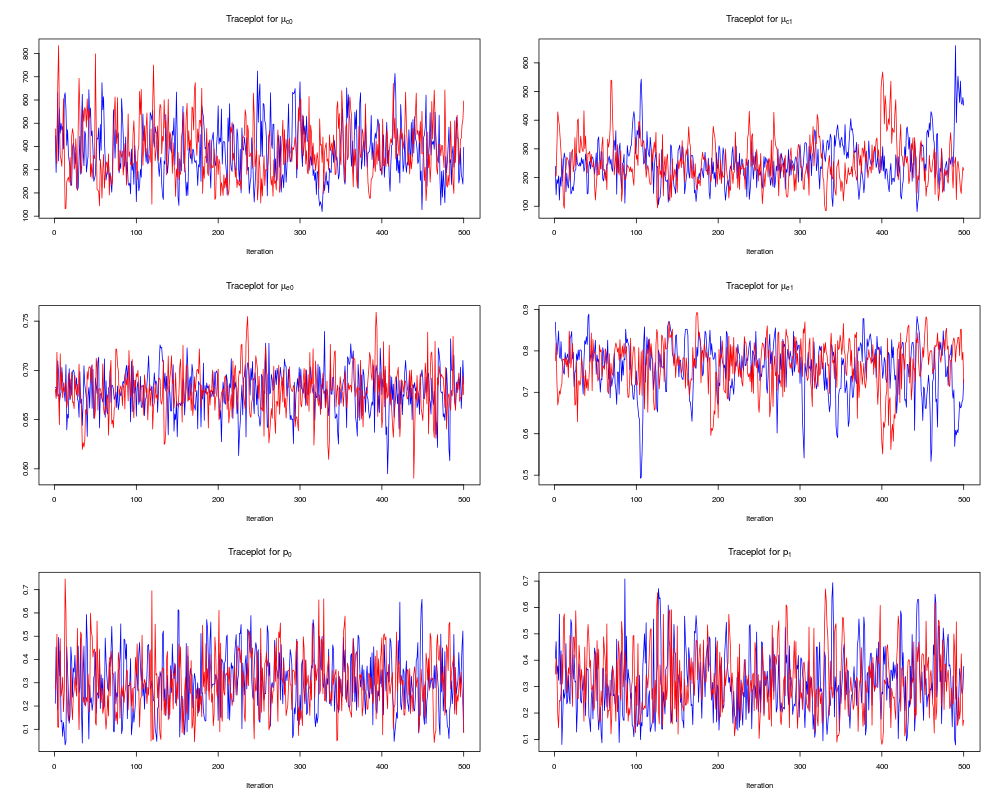
mu.c[1] 383.755 123.298 164.535 635.988 1.001 1000
mu.c[2] 247.829 67.265 133.981 396.223 1.000 1000
mu.e[1] 0.679 0.022 0.633 0.719 1.002 1000
mu.e[2] 0.769 0.053 0.656 0.858 1.003 1000
p[1] 0.293 0.133 0.082 0.598 1.000 1000
p[2] 0.326 0.120 0.119 0.571 1.000 1000
psi0[1] 541.102 135.188 274.181 808.251 1.003 560
psi0[2] 0.000 0.000 0.000 0.000 1.000 1
psi1[1] 368.466 80.825 243.376 573.976 1.000 1000
psi1[2] 0.000 0.000 0.000 0.000 1.000 1
tau0 53.915 27.544 15.526 121.921 1.008 180
tau1 6.292 2.521 2.523 12.421 1.026 88
deviance 29.502 5.273 21.410 42.268 1.007 200
For each parameter, n.eff is a crude measure of effective sample size,
and Rhat is the potential scale reduction factor (at convergence, Rhat=1).
DIC info (using the rule, pD = var(deviance)/2)
pD = 13.9 and DIC = 43.4
DIC is an estimate of expected predictive error (lower deviance is better).
> plot(m)
>
>
>
>
>
> dev.off()
null device
1
>
 .
.