R: Bayesian parameter estimation for discrete Weibull regression
bdw
R Documentation
Bayesian parameter estimation for discrete Weibull regression
Description
Bayesian estimation of the parameters for discrete Weibull regression. The conditional distribution of the response given the predictors is assumed to be DW with parameters q and beta dependent on the predictors.
A data frame containing the variables in the model. If not found in data, the variables are taken from the environment (formula).
formula
An object of class "formula". A symbolic description of the model to be fitted.
reg.q
Logical flag. If TRUE, the model includes a dependency of q on the predictors x, as explained in 'logit' argument.
reg.b
Logical flag. If TRUE, the model includes a dependency of beta on the predictors x, given by:
log(β)= γ_0+γ_1X_1+…+γ_pX_p.
If FALSE, beta(x) is constant.
logit
Logical flag. If TRUE, the model includes a dependency of q on predictors via a logit transformation as explained below.
The conditional distribution of Y (response) given x (predictors) is assumed a DW(q(x),beta(x)).
If logit=TRUE & (reg.q=TRUE)
log(q/(1-q))=θ_0+θ_1 X_1+…+θ_pX_p.
If logit=FALSE & (reg.q=TRUE)
log(-log(q))=θ_0+θ_1 X_1+…+θ_pX_p.
initial
Vector of initial values for parameters. In all cases DW(q,B), DW(regQ,B), DW(q,rebB) and DW(regQ,regB) the first parameters correspond to q or corresponding regression coefficients and next is beta or corresponding regression coefficients. If penalized=TRUE then an extra value must be added for tunning parameter.
iteration
Number of MCMC iterations.
v.scale
The scale of the proposal function. Setting to lower values results in an increase in the acceptance rate of the sampler.
RJ
Logical flag. If TRUE, Reversible-Jump sampling is used to draw samples from the posterior. Otherwise, a Metropolis-Hasting sampler applies.
dist.q
Density function. Prior density for theta. If not set, an improper prior applies. Any two parameter density function is allowed, e.g. dnorm, dlaplace, dunif etc. Any customized density function must support log=TRUE flag.
dist.b
Density function. Prior density for gamma. If not set, an improper prior applies. Any two parameter density function is allowed, e.g. dnorm, dlaplace, dunif etc. Any customized density function must support log=TRUE flag.
q.par
A vector of length two corresponding to the parameters of 'dist.q'. The default is set to c(0,0).
b.par
A vector of length two corresponding to the parameters of 'dist.b'. The default is set to c(0,0).
penalized
logical flag. If TRUE, an hyper-parameter inducing shrinkage is considered. In this case, priors must be set to an informative prior, e.g. Gaussian, Laplace. See also 'l.par' and 'dist.l' below.
dist.l
Density function. Hyper prior for penalty term. If not set, an improper prior is used. Any non-negative two parameter density function is allowed, e.g. dgamma, dbeta,... Any customized density function must support log=TRUE flag.
l.par
A vector of length two corresponding to the parameters of the hyperprior 'dist.l'. The default is set to c(0,0).
bi.period
A numeric value in (0,1) indicating the burn-in period of the MCMC chain. The default is set to 0.25 meaning that 25% of values remove from the beginning of the output chain. See 'sampling'.
cov
A value in {1,2,3,4}. If set to 1 then the correlation among chains is considered in the proposal; 2: an independent uniform proposal; 3: an independent Laplace proposal and 4: an independent Gaussian proposal. The default is 1.
sampling
Choose between independent (indp), systematic (syst) and burn-in (bin). If set to indp then the chain is not ordered! The default is 'bin'. Sampling interval for Systematic sampling is calculated from iteration(1-bi.period). Similarly for indp the number of samples is computed from iteration(1-bi.period).
est
Statistic. The statistic that is used to estimate the parameters from marginal densities. Possible values are: mode, mean, median or any customized univariate measure of location. The default is 'mode'.
fixed.l
A positive number. Set to a positive value corresponding to a parameter that does not need estimation. Set to any negative value to disable this option.
...
Value
res
Estimation of the parameters from marginal densities using the statistic specified in 'est' .
chain
A list of values including sampler configurations.
chain : Including estimation of marginal densities
acceptance.rate: Acceptance rate of sampler
RejAccChain : A zero-one vector reporting rejection (0) and acceptance (1) of the samples
error : Total number of errors during the sampling procedure
minf : Minimum loglikelihood among all iterations
minState : Coefficients corresponding to minimum loglikelihood
lb : The number of gamma parameters
lq : The number of theta parameters
model.chain : If RJ=TRUE then this chain contains acceptance (+values) and rejection (-values) of models
duration : Time elapsed until completion of the sampling procedure
Author(s)
Hamed Haselimashhadi <hamedhaseli@gmail.com>
References
Haselimashhadi, Vinciotti and Yu (2015), A new Bayesian regression model for counts in medicine.
See Also
plot.bdw,
summary.bdw,
bdw.mc
Examples
set.seed(123)
#========== example 1 - estimating DW parameters under logit transformation ==========
q = .41    # <<< true parameters
b = 1.1    # <<< true parameters
y = BDWreg:::rdw(n = 200,q = q,beta = b) #<<< generating data
result  = bdw(data = y, v.scale = .10,initial = c(.5,.5),iteration = 8000 )
plot(result)
summary(result)


## Not run:
  #==== example 2 - estimating logit-DW(regQ,beta) parameters using RJ ======
  set.seed(1234)
  n = 500
  x1 = runif(n = n, min = 0, max = 1.5)
  x2 = runif(n = n, min = 0, max = 1.5)

  theta0 = .6   #<<< true parameter
  theta1 =  0   #<<< true parameter
  theta2 = .34  #<<< true parameter

  lq = theta0 +  x1*theta1 + x2*theta2

  q = exp(lq - log(1+exp(lq)) )
  beta = 1.5

  y = c()
  for(i in 1:n){
    y[i] = BDWreg:::rdw(1,q = q[i],beta = beta)
  }

  data = data.frame(x1,x2,y) # <<<- data
  result2 = bdw(data = data              ,
               formula = y~.             ,
               RJ = TRUE                 ,
               initial = rep(.5,4)       ,
               iteration = 25000         ,
               reg.b = FALSE,reg.q = TRUE,
               v.scale = .1              ,
               q.par = c(0,1)            ,
               b.par = c(0,1)            ,
               dist.q = dnorm            ,
               dist.b = dnorm
  )
  plot(result2)
  summary(result2)

## End(Not run)
Results
R version 3.3.1 (2016-06-21) -- "Bug in Your Hair"
Copyright (C) 2016 The R Foundation for Statistical Computing
Platform: x86_64-pc-linux-gnu (64-bit)
R is free software and comes with ABSOLUTELY NO WARRANTY.
You are welcome to redistribute it under certain conditions.
Type 'license()' or 'licence()' for distribution details.
R is a collaborative project with many contributors.
Type 'contributors()' for more information and
'citation()' on how to cite R or R packages in publications.
Type 'demo()' for some demos, 'help()' for on-line help, or
'help.start()' for an HTML browser interface to help.
Type 'q()' to quit R.
> library(BDWreg)
========================================================================
If you have any question about this package and corresponding paper use
hamedhaseli@gmail.com or visit www.hamedhaseli.webs.com
========================================================================
> png(filename="/home/ddbj/snapshot/RGM3/R_CC/result/BDWreg/bdw.Rd_%03d_medium.png", width=480, height=480)
> ### Name: bdw
> ### Title: Bayesian parameter estimation for discrete Weibull regression
> ### Aliases: bdw
> ### Keywords: Discrete Weibull regression Reversible-Jumps
> ### Metropolise-Hasings
>
> ### ** Examples
>
> set.seed(123)
> #========== example 1 - estimating DW parameters under logit transformation ==========
> q = .41 # <<< true parameters
> b = 1.1 # <<< true parameters
> y = BDWreg:::rdw(n = 200,q = q,beta = b) #<<< generating data
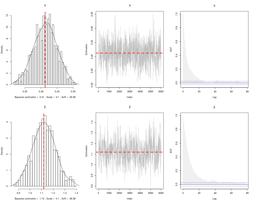
> result = bdw(data = y, v.scale = .10,initial = c(.5,.5),iteration = 8000 )
============================== Sampler configuration ==============================
Iterations: 8000 | Data: FALSE | Length of Initials: 2
RegQ: FALSE | RegB: FALSE | Formula: FALSE
Logit: TRUE | Scale: 0.1 | Rev.Jumps: FALSE
Penalized: FALSE | Fixed.penalty: FALSE |
----------------------------------------------------------------------------------
Proposal (1=Including covariates,2=Uniform,3=Laplace,>3=Gaussian): 1
----------------------------------------------------------------------------------
Chain summary (bin=Burn-in, syst=Systematic, indp=Independent): bin
----------------------------------------------------------------------------------
* If Penalized=TRUE then you need to set all distributions.
----------------------------------------------------------------------------------
* If RJ=TRUE then Penalized is automatically set to FALSE and fixed.l diactivates.
__________________________________________________________________________________
5 % done, Acceptance = 1 % 10 % done, Acceptance = 2.27 % 15 % done, Acceptance = 3.67 % 20 % done, Acceptance = 5 % 25 % done, Acceptance = 6.22 % 30 % done, Acceptance = 7.26 % 35 % done, Acceptance = 8.61 % 40 % done, Acceptance = 9.91 % 45 % done, Acceptance = 11.15 % 50 % done, Acceptance = 12.52 % 55 % done, Acceptance = 13.8 % 60 % done, Acceptance = 15.11 % 65 % done, Acceptance = 16.42 % 70 % done, Acceptance = 17.7 % 75 % done, Acceptance = 19.2 % 80 % done, Acceptance = 20.71 % 85 % done, Acceptance = 22.18 % 90 % done, Acceptance = 23.47 % 95 % done, Acceptance = 24.93 % 100 % done, Acceptance = 26.13 %
There are 721 ignored values in the process!
Procedure finished in 3.08 seconds.
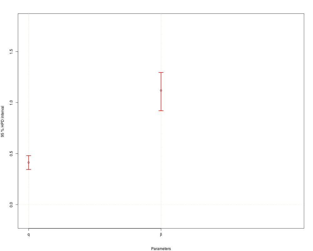
> plot(result)
Loading required namespace: coda
1 of 2 plot completed. 2 of 2 plot completed.
======= 95 % Confidence interval =======
lower est upper Zero.included
q 0.3444707 0.4126489 0.4800809 0
B 0.9207588 1.1191823 1.2950023 0
> summary(result)
Please wait ...
============================== Sampler ================================
Iterations : 8000 Logit : TRUE Scale : 0.1
Rev.Jump : FALSE RegQ : FALSE RegB : FALSE
Penalized : FALSE Fixed.penalty : FALSE
============================ Model Summary ============================
AIC : 435.7952 AICc : 435.8555 BIC : 442.3918
QIC : 2.172839 CAIC : 444.3918 LogPPD : -218.4877
DIC : 436.0942 PBIC : 438.238 df : 2
=======================================================================
>
>
> ## Not run:
> ##D #==== example 2 - estimating logit-DW(regQ,beta) parameters using RJ ======
> ##D set.seed(1234)
> ##D n = 500
> ##D x1 = runif(n = n, min = 0, max = 1.5)
> ##D x2 = runif(n = n, min = 0, max = 1.5)
> ##D
> ##D theta0 = .6 #<<< true parameter
> ##D theta1 = 0 #<<< true parameter
> ##D theta2 = .34 #<<< true parameter
> ##D
> ##D lq = theta0 + x1*theta1 + x2*theta2
> ##D
> ##D q = exp(lq - log(1+exp(lq)) )
> ##D beta = 1.5
> ##D
> ##D y = c()
> ##D for(i in 1:n){
> ##D y[i] = BDWreg:::rdw(1,q = q[i],beta = beta)
> ##D }
> ##D
> ##D data = data.frame(x1,x2,y) # <<<- data
> ##D result2 = bdw(data = data ,
> ##D formula = y~. ,
> ##D RJ = TRUE ,
> ##D initial = rep(.5,4) ,
> ##D iteration = 25000 ,
> ##D reg.b = FALSE,reg.q = TRUE,
> ##D v.scale = .1 ,
> ##D q.par = c(0,1) ,
> ##D b.par = c(0,1) ,
> ##D dist.q = dnorm ,
> ##D dist.b = dnorm
> ##D )
> ##D plot(result2)
> ##D summary(result2)
> ## End(Not run)
>
>
>
>
>
> dev.off()
null device
1
>
 .
.