Summary for a MCMC object of class 'bdw'

Description

This function produces result summaries from a MCMC object of class 'bdw'

Usage

## S3 method for class 'bdw'
summary(object, est = Mode, prob = 0.95, samp = TRUE, ...)

Arguments

Author(s)

Hamed Haselimashhadi <hamedhaseli@gmail.com>

See Also

bdw, plot.bdw, bdw.mc

Examples

example(bdw)

Results

R version 3.3.1 (2016-06-21) -- "Bug in Your Hair"
Copyright (C) 2016 The R Foundation for Statistical Computing
Platform: x86_64-pc-linux-gnu (64-bit)

R is free software and comes with ABSOLUTELY NO WARRANTY.
You are welcome to redistribute it under certain conditions.
Type 'license()' or 'licence()' for distribution details.

R is a collaborative project with many contributors.
Type 'contributors()' for more information and
'citation()' on how to cite R or R packages in publications.

Type 'demo()' for some demos, 'help()' for on-line help, or
'help.start()' for an HTML browser interface to help.
Type 'q()' to quit R.

> library(BDWreg)

 ========================================================================
 If you have any question about this package and corresponding paper use 
      hamedhaseli@gmail.com  or visit www.hamedhaseli.webs.com           
 ========================================================================
> png(filename="/home/ddbj/snapshot/RGM3/R_CC/result/BDWreg/summary.bdw.Rd_%03d_medium.png", width=480, height=480)
> ### Name: summary.bdw
> ### Title: Summary for a MCMC object of class 'bdw'
> ### Aliases: summary.bdw
> 
> ### ** Examples
> 
> example(bdw)

bdw> set.seed(123)

bdw> #========== example 1 - estimating DW parameters under logit transformation ==========
bdw> q = .41    # <<< true parameters

bdw> b = 1.1    # <<< true parameters

bdw> y = BDWreg:::rdw(n = 200,q = q,beta = b) #<<< generating data

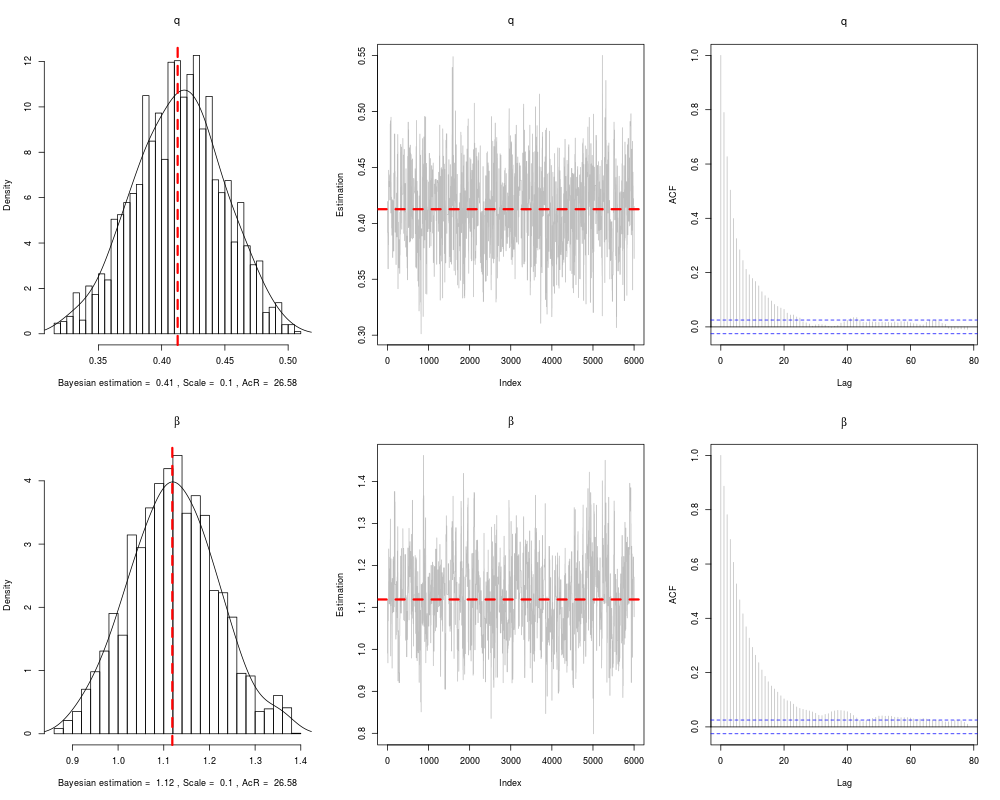
bdw> result  = bdw(data = y, v.scale = .10,initial = c(.5,.5),iteration = 8000 )


============================== Sampler configuration ============================== 
Iterations: 8000 	| Data: FALSE 	 	| Length of Initials: 2 
RegQ: FALSE 	 	| RegB: FALSE 	 	| Formula: FALSE 
Logit: TRUE 	 	| Scale: 0.1 		| Rev.Jumps: FALSE 
Penalized: FALSE 	| Fixed.penalty: FALSE  |	 
----------------------------------------------------------------------------------   
Proposal (1=Including covariates,2=Uniform,3=Laplace,>3=Gaussian): 1 
----------------------------------------------------------------------------------   
Chain summary (bin=Burn-in, syst=Systematic, indp=Independent): bin 
----------------------------------------------------------------------------------   
* If Penalized=TRUE then you need to set all distributions.                
----------------------------------------------------------------------------------   
* If RJ=TRUE then Penalized is automatically set to FALSE and fixed.l diactivates. 
__________________________________________________________________________________  
   5 % done, Acceptance =  1 %   10 % done, Acceptance =  2.27 %   15 % done, Acceptance =  3.67 %   20 % done, Acceptance =  5 %   25 % done, Acceptance =  6.22 %   30 % done, Acceptance =  7.26 %   35 % done, Acceptance =  8.61 %   40 % done, Acceptance =  9.91 %   45 % done, Acceptance =  11.15 %   50 % done, Acceptance =  12.52 %   55 % done, Acceptance =  13.8 %   60 % done, Acceptance =  15.11 %   65 % done, Acceptance =  16.42 %   70 % done, Acceptance =  17.7 %   75 % done, Acceptance =  19.2 %   80 % done, Acceptance =  20.71 %   85 % done, Acceptance =  22.18 %   90 % done, Acceptance =  23.47 %   95 % done, Acceptance =  24.93 %   100 % done, Acceptance =  26.13 % 

 There are  721  ignored values in the process!
 Procedure finished in  2.616  seconds. 

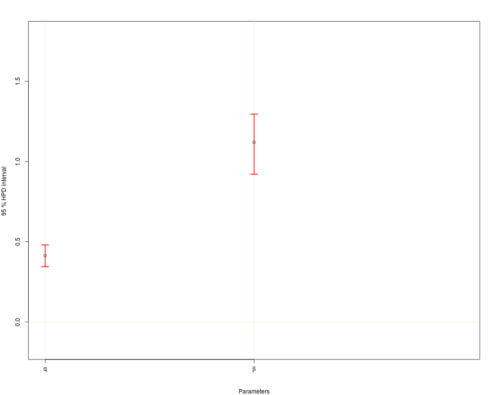
bdw> plot(result)
Loading required namespace: coda
  1  of  2  plot completed.  2  of  2  plot completed.
 ======= 95 % Confidence interval ======= 
      lower       est     upper Zero.included
q 0.3444707 0.4126489 0.4800809             0
B 0.9207588 1.1191823 1.2950023             0

bdw> summary(result)
  Please wait ... 
 ============================== Sampler ================================ 
     Iterations :  8000 	 Logit :  TRUE 	 Scale :  0.1 
     Rev.Jump   :  FALSE 	 RegQ  :  FALSE 	 RegB  :  FALSE 
     Penalized  :  FALSE 	 Fixed.penalty :  FALSE 
 ============================ Model Summary ============================ 
     AIC :  435.7952 	 AICc :  435.8555 	 BIC     :  442.3918 
     QIC :  2.172839 	 CAIC :  444.3918 	 LogPPD  :  -218.4877 
     DIC :  436.0942 	 PBIC :  438.238 	 df      :  2 
 =======================================================================  

bdw> ## Not run: 
bdw> ##D   #==== example 2 - estimating logit-DW(regQ,beta) parameters using RJ ======
bdw> ##D   set.seed(1234)
bdw> ##D   n = 500
bdw> ##D   x1 = runif(n = n, min = 0, max = 1.5)
bdw> ##D   x2 = runif(n = n, min = 0, max = 1.5)
bdw> ##D 
bdw> ##D   theta0 = .6   #<<< true parameter
bdw> ##D   theta1 =  0   #<<< true parameter
bdw> ##D   theta2 = .34  #<<< true parameter
bdw> ##D 
bdw> ##D   lq = theta0 +  x1*theta1 + x2*theta2
bdw> ##D 
bdw> ##D   q = exp(lq - log(1+exp(lq)) )
bdw> ##D   beta = 1.5
bdw> ##D 
bdw> ##D   y = c()
bdw> ##D   for(i in 1:n){
bdw> ##D     y[i] = BDWreg:::rdw(1,q = q[i],beta = beta)
bdw> ##D   }
bdw> ##D 
bdw> ##D   data = data.frame(x1,x2,y) # <<<- data
bdw> ##D   result2 = bdw(data = data              ,
bdw> ##D                formula = y~.             ,
bdw> ##D                RJ = TRUE                 ,
bdw> ##D                initial = rep(.5,4)       ,
bdw> ##D                iteration = 25000         ,
bdw> ##D                reg.b = FALSE,reg.q = TRUE,
bdw> ##D                v.scale = .1              ,
bdw> ##D                q.par = c(0,1)            ,
bdw> ##D                b.par = c(0,1)            ,
bdw> ##D                dist.q = dnorm            ,
bdw> ##D                dist.b = dnorm
bdw> ##D   )
bdw> ##D   plot(result2)
bdw> ##D   summary(result2)
bdw> ## End(Not run)
bdw> 
bdw> 
bdw> 
> 
> 
> 
> 
> 
> dev.off()
null device 
          1 
>