Bayesian Estimation Supersedes the t Test

Description

An alternative to t tests, producing posterior estimates for groups means and standard deviations and their differences and effect sizes. Bayesian estimation provides a much richer picture of the data, and can be summarised as point estimates and credible intervals.

Details

The core function, BESTmcmc, generates posterior distributions to compare the means of two groups, or to compare the mean of one group with a standard, taking into account the standard deviation(s). It is thus similar to a t test. However, our Bayesian approach results in probability statements about the values of interest, rather than p-values and significance levels.

In addition, the procedure accounts for departures from normality by using a t-distribution to model the variable of interest and estimating a measure of normality.

Functions to summarise and to visualise the output are provided.

The function BESTpower allows simulation-based estimates of power, either retrospective power directly with BESTmcmc output or prospective power analysis with makeData.

Author(s)

Original code by John K. Kruschke, http://www.indiana.edu/~kruschke/BEST/

Maintainer: Mike Meredith <mmeredith at wcs.org>

References

Kruschke, J. K. 2013. Bayesian estimation supersedes the t test. Journal of Experimental Psychology: General 142(2):573-603. doi: 10.1037/a0029146

Kruschke, J. K. 2011. Doing Bayesian data analysis: a tutorial with R and BUGS. Elsevier, Amsterdam, especially Chapter 18.

Examples

## Comparison of two groups:
## =========================
y1 <- c(5.77, 5.33, 4.59, 4.33, 3.66, 4.48)
y2 <- c(3.88, 3.55, 3.29, 2.59, 2.33, 3.59)

# Run an analysis, takes up to 1 min.
BESTout <- BESTmcmc(y1, y2)

# Look at the result:
BESTout
summary(BESTout)
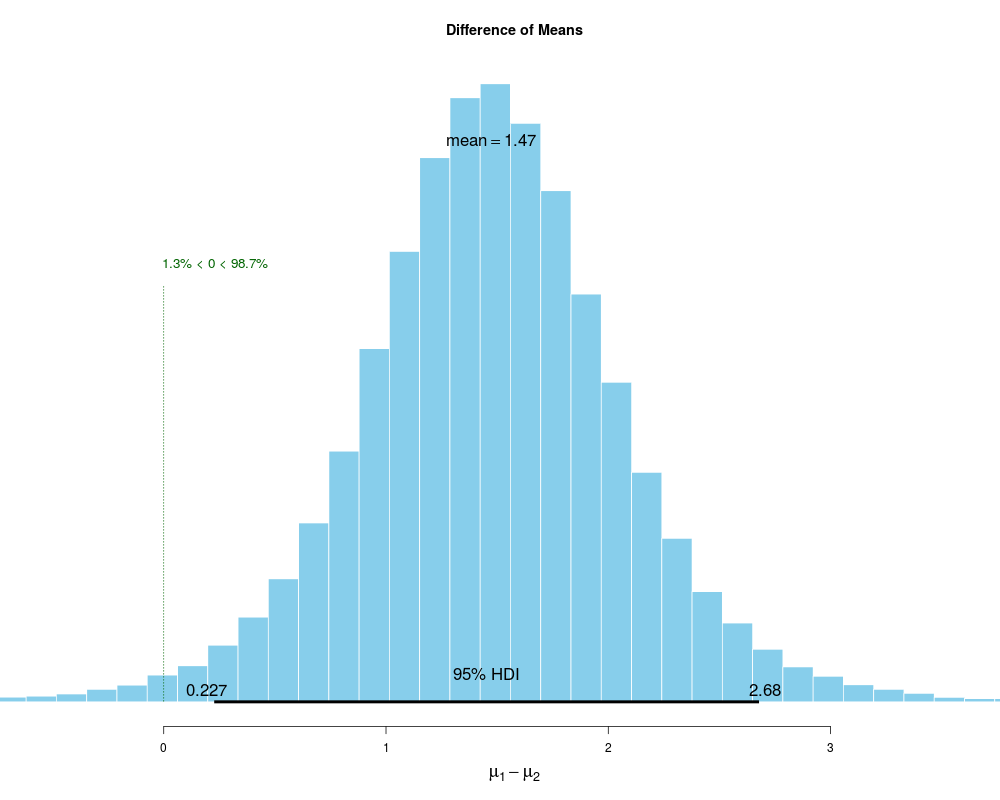
plot(BESTout)
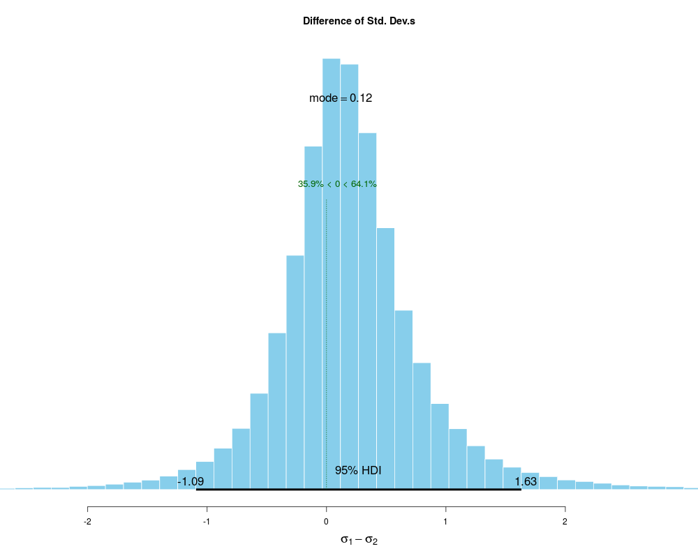
plot(BESTout, "sd")
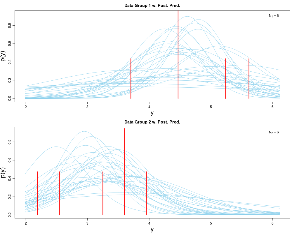
plotPostPred(BESTout)
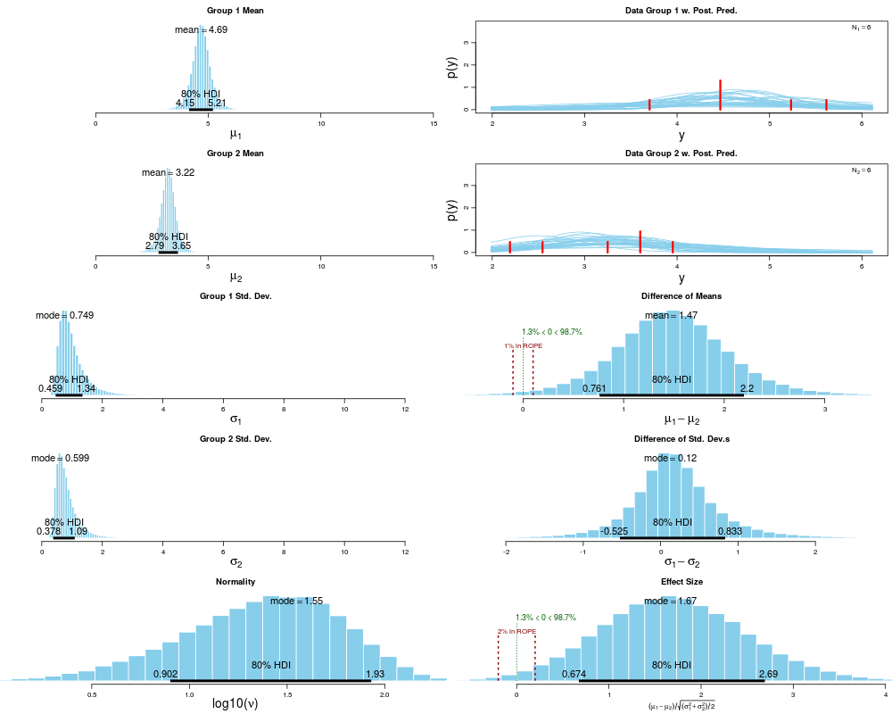
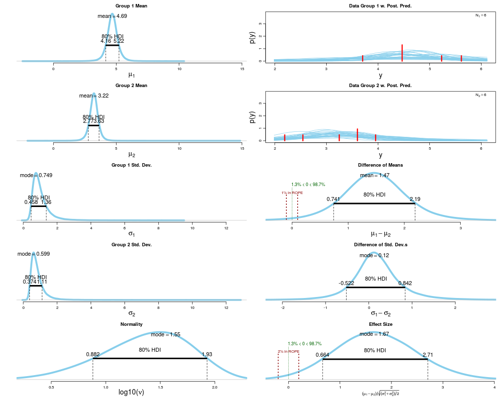
plotAll(BESTout, credMass=0.8, ROPEm=c(-0.1,0.1), 
          ROPEeff=c(-0.2,0.2), compValm=0.5) 
plotAll(BESTout, credMass=0.8, ROPEm=c(-0.1,0.1), 
          ROPEeff=c(-0.2,0.2), compValm=0.5, showCurve=TRUE) 
summary(BESTout, credMass=0.8, ROPEm=c(-0.1,0.1), ROPEsd=c(-0.15,0.15),
          ROPEeff=c(-0.2,0.2)) 
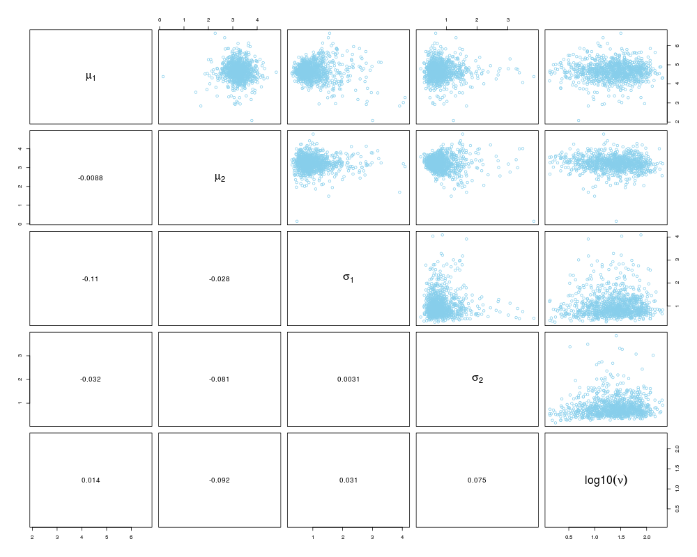
pairs(BESTout)

head(BESTout$mu1)
muDiff <- BESTout$mu1 - BESTout$mu2
mean(muDiff > 1.5)
mean(BESTout$sigma1 - BESTout$sigma2)
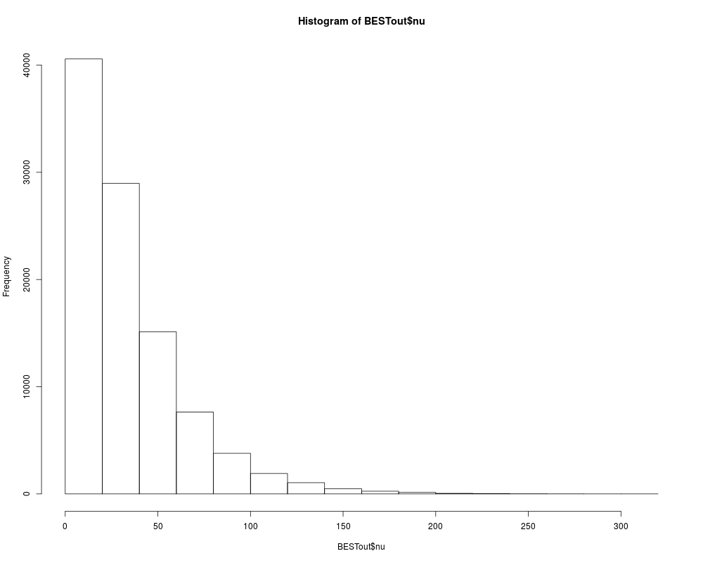
hist(BESTout$nu)

# Retrospective power analysis
# ----------------------------
# This takes time, so we do 2 simulations here; a real analysis needs several hundred

powerRet <- BESTpower(BESTout, N1=length(y1), N2=length(y2), 
            ROPEm=c(-0.1,0.1), maxHDIWm=2.0, nRep=2) 
powerRet
# We only set criteria for the mean, so results for sd and effect size are all NA.

## Analysis with a single group:
## =============================
y0 <- c(1.89, 1.78, 1.30, 1.74, 1.33, 0.89)

# Run an analysis, takes up to 40 secs.
BESTout1 <- BESTmcmc(y0)
BESTout1
summary(BESTout1)
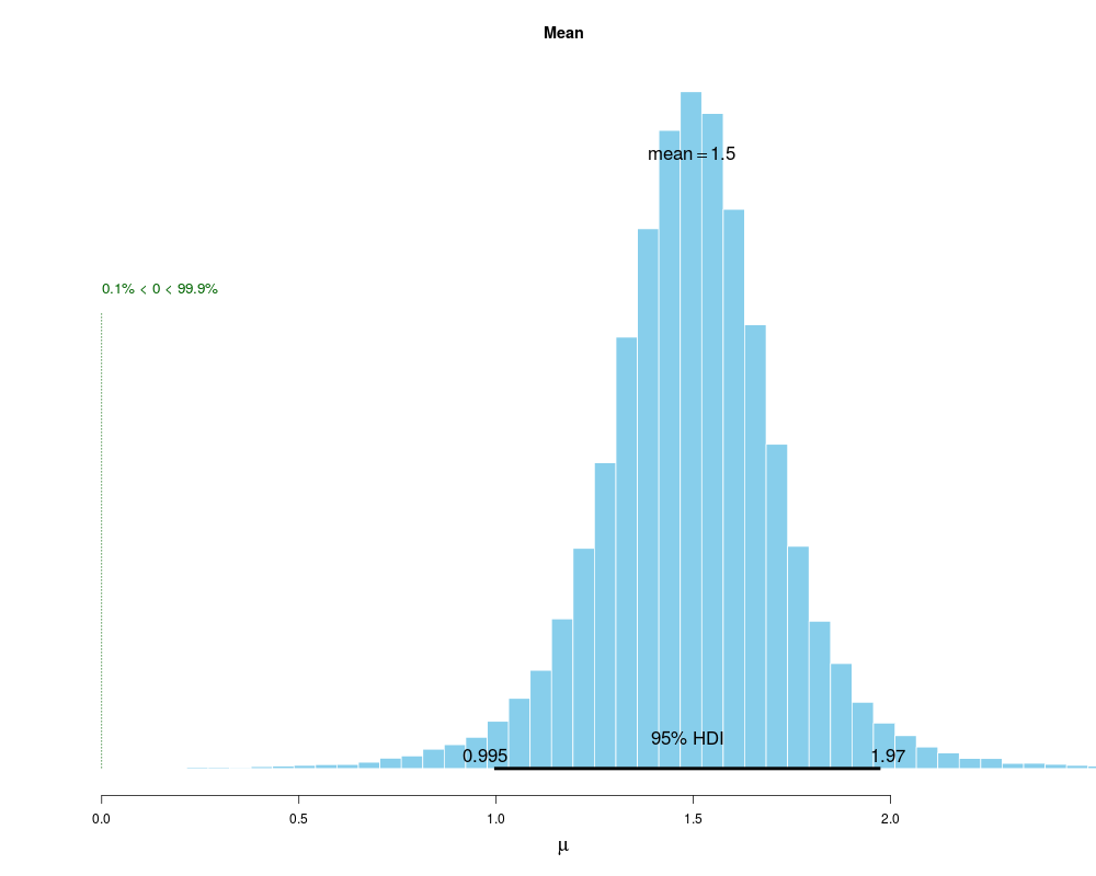
plot(BESTout1)

head(BESTout1$mu)
mean(BESTout1$sigma)
 

Results

R version 3.3.1 (2016-06-21) -- "Bug in Your Hair"
Copyright (C) 2016 The R Foundation for Statistical Computing
Platform: x86_64-pc-linux-gnu (64-bit)

R is free software and comes with ABSOLUTELY NO WARRANTY.
You are welcome to redistribute it under certain conditions.
Type 'license()' or 'licence()' for distribution details.

R is a collaborative project with many contributors.
Type 'contributors()' for more information and
'citation()' on how to cite R or R packages in publications.

Type 'demo()' for some demos, 'help()' for on-line help, or
'help.start()' for an HTML browser interface to help.
Type 'q()' to quit R.

> library(BEST)
> png(filename="/home/ddbj/snapshot/RGM3/R_CC/result/BEST/BEST-package.Rd_%03d_medium.png", width=480, height=480)
> ### Name: BEST-package
> ### Title: Bayesian Estimation Supersedes the t Test
> ### Aliases: BEST-package BEST
> ### Keywords: package htest
> 
> ### ** Examples
> 
> 
> ## No test: 
> ## Comparison of two groups:
> ## =========================
> y1 <- c(5.77, 5.33, 4.59, 4.33, 3.66, 4.48)
> y2 <- c(3.88, 3.55, 3.29, 2.59, 2.33, 3.59)
> 
> # Run an analysis, takes up to 1 min.
> BESTout <- BESTmcmc(y1, y2)

Processing function input....... 

Done. 
 
Beginning parallel processing using 3 cores. Console output will be suppressed.

Parallel processing completed.

MCMC took 0.088 minutes.
> 
> # Look at the result:
> BESTout
MCMC fit results for BEST analysis:
100002 simulations saved.
          mean      sd  median  HDIlo  HDIup  Rhat n.eff
mu1     4.6880  0.4938  4.6842 3.7416  5.623 1.006 30831
mu2     3.2166  0.3958  3.2209 2.4345  3.982 1.000 30077
nu     33.4806 29.1211 25.1112 1.0144 91.328 1.000 20431
sigma1  1.0198  0.5462  0.8845 0.3578  2.014 1.005  9622
sigma2  0.8371  0.4339  0.7290 0.3059  1.645 1.001  9122

'HDIlo' and 'HDIup' are the limits of a 95% HDI credible interval.
'Rhat' is the potential scale reduction factor (at convergence, Rhat=1).
'n.eff' is a crude measure of effective sample size.
> summary(BESTout)
            mean median  mode HDI%  HDIlo HDIup compVal %>compVal
mu1        4.688  4.684 4.662   95  3.742  5.62                  
mu2        3.217  3.221 3.244   95  2.435  3.98                  
muDiff     1.471  1.467 1.500   95  0.228  2.68       0      98.7
sigma1     1.020  0.885 0.722   95  0.358  2.01                  
sigma2     0.837  0.729 0.604   95  0.306  1.64                  
sigmaDiff  0.183  0.148 0.124   95 -1.106  1.63       0      63.7
nu        33.481 25.111 8.858   95  1.014 91.33                  
log10nu    1.362  1.400 1.495   95  0.549  2.09                  
effSz      1.702  1.680 1.626   95  0.179  3.30       0      98.7
> plot(BESTout)
> plot(BESTout, "sd")
> plotPostPred(BESTout)
> plotAll(BESTout, credMass=0.8, ROPEm=c(-0.1,0.1), 
+           ROPEeff=c(-0.2,0.2), compValm=0.5) 
> plotAll(BESTout, credMass=0.8, ROPEm=c(-0.1,0.1), 
+           ROPEeff=c(-0.2,0.2), compValm=0.5, showCurve=TRUE) 
> summary(BESTout, credMass=0.8, ROPEm=c(-0.1,0.1), ROPEsd=c(-0.15,0.15),
+           ROPEeff=c(-0.2,0.2)) 
            mean median  mode HDI%  HDIlo  HDIup compVal %>compVal ROPElow
mu1        4.688  4.684 4.662   80  4.146  5.195                          
mu2        3.217  3.221 3.244   80  2.794  3.653                          
muDiff     1.471  1.467 1.500   80  0.729  2.161       0      98.7   -0.10
sigma1     1.020  0.885 0.722   80  0.454  1.335                          
sigma2     0.837  0.729 0.604   80  0.368  1.087                          
sigmaDiff  0.183  0.148 0.124   80 -0.532  0.828       0      63.7   -0.15
nu        33.481 25.111 8.858   80  1.418 52.029                          
log10nu    1.362  1.400 1.495   80  0.884  1.910                          
effSz      1.702  1.680 1.626   80  0.663  2.692       0      98.7   -0.20
          ROPEhigh %InROPE
mu1                       
mu2                       
muDiff        0.10   0.666
sigma1                    
sigma2                    
sigmaDiff     0.15  25.478
nu                        
log10nu                   
effSz         0.20   1.925
> pairs(BESTout)
> 
> head(BESTout$mu1)
[1] 4.616803 4.916176 4.669184 4.562231 5.138517 5.147933
> muDiff <- BESTout$mu1 - BESTout$mu2
> mean(muDiff > 1.5)
[1] 0.4755205
> mean(BESTout$sigma1 - BESTout$sigma2)
[1] 0.182755
> hist(BESTout$nu)
> 
> # Retrospective power analysis
> # ----------------------------
> # This takes time, so we do 2 simulations here; a real analysis needs several hundred
> 
> powerRet <- BESTpower(BESTout, N1=length(y1), N2=length(y2), 
+             ROPEm=c(-0.1,0.1), maxHDIWm=2.0, nRep=2) 

:::::::::::::::::::::::::::::::::::::::::::::::::::::::::::::::
Power computation: Simulated Experiment 1 of 2 :


Processing function input....... 

Done. 
 
Beginning parallel processing using 3 cores. Console output will be suppressed.

Parallel processing completed.

MCMC took 0.035 minutes.

After 1 Simulated Experiments, Posterior Probability
         of meeting each criterion is (mean and 95% CrI):
                      mean CrIlo CrIhi
  mean:   HDI > ROPE 0.333     0 0.776
  mean:   HDI < ROPE 0.333     0 0.776
  mean:  HDI in ROPE 0.333     0 0.776
  mean: HDI width ok 0.333     0 0.776

:::::::::::::::::::::::::::::::::::::::::::::::::::::::::::::::
Power computation: Simulated Experiment 2 of 2 :


Processing function input....... 

Done. 
 
Beginning parallel processing using 3 cores. Console output will be suppressed.

Parallel processing completed.

MCMC took 0.03 minutes.

After 2 Simulated Experiments, Posterior Probability
         of meeting each criterion is (mean and 95% CrI):
                     mean CrIlo CrIhi
  mean:   HDI > ROPE 0.25     0 0.632
  mean:   HDI < ROPE 0.25     0 0.632
  mean:  HDI in ROPE 0.25     0 0.632
  mean: HDI width ok 0.25     0 0.632
> powerRet
                     mean        CrIlo     CrIhi
  mean:   HDI > ROPE 0.25 2.114738e-09 0.6315969
  mean:   HDI < ROPE 0.25 2.114738e-09 0.6315969
  mean:  HDI in ROPE 0.25 2.114738e-09 0.6315969
  mean: HDI width ok 0.25 2.114738e-09 0.6315969
    sd:   HDI > ROPE   NA           NA        NA
    sd:   HDI < ROPE   NA           NA        NA
    sd:  HDI in ROPE   NA           NA        NA
    sd: HDI width ok   NA           NA        NA
effect:   HDI > ROPE   NA           NA        NA
effect:   HDI < ROPE   NA           NA        NA
effect:  HDI in ROPE   NA           NA        NA
effect: HDI width ok   NA           NA        NA
> # We only set criteria for the mean, so results for sd and effect size are all NA.
> 
> ## Analysis with a single group:
> ## =============================
> y0 <- c(1.89, 1.78, 1.30, 1.74, 1.33, 0.89)
> 
> # Run an analysis, takes up to 40 secs.
> BESTout1 <- BESTmcmc(y0)

Processing function input....... 

Done. 
 
Beginning parallel processing using 3 cores. Console output will be suppressed.

Parallel processing completed.

MCMC took 0.074 minutes.
> BESTout1
MCMC fit results for BEST analysis:
100002 simulations saved.
         mean      sd  median  HDIlo  HDIup  Rhat n.eff
mu     1.4970  0.2689  1.4970 0.9901  1.963 1.014 17869
nu    32.3996 29.8412 23.3732 1.0003 91.703 1.000 18480
sigma  0.5278  0.3307  0.4518 0.1851  1.033 1.036  3865

'HDIlo' and 'HDIup' are the limits of a 95% HDI credible interval.
'Rhat' is the potential scale reduction factor (at convergence, Rhat=1).
'n.eff' is a crude measure of effective sample size.
> summary(BESTout1)
          mean median  mode HDI% HDIlo HDIup compVal %>compVal
mu       1.497  1.497 1.492   95 0.990  1.96       0      99.9
sigma    0.528  0.452 0.371   95 0.185  1.03                  
nu      32.400 23.373 7.314   95 1.000 91.70                  
log10nu  1.329  1.369 1.450   95 0.449  2.09                  
effSz    3.444  3.315 3.010   95 0.831  6.24       0      99.9
> plot(BESTout1)
> 
> head(BESTout1$mu)
[1] 1.712800 1.699769 1.745293 1.797035 1.418139 1.592211
> mean(BESTout1$sigma)
[1] 0.5277566
> ## End(No test) 
> 
> 
> 
> 
> 
> dev.off()
null device 
          1 
>