R Graphical Manual

Browse All

Last data update: 2014.03.03

R: Estimating statistical power

BESTpower

R Documentation

Estimating statistical power

Description

Estimation of the probability of meeting the goals of a study given initial information or assumptions about the population parameters. For prospective power estimation, the sequence
makeData -> BESTmcmc -> BESTpower
is recommended: see makeData.

Usage

BESTpower(BESTobj, N1, N2, credMass=0.95,
 ROPEm, ROPEsd, ROPEeff, 
 maxHDIWm, maxHDIWsd, maxHDIWeff,
 compValm = 0, nRep = 200, mcmcLength = 10000,
 saveName = NULL, showFirstNrep = 0, verbose = 2, rnd.seed=NULL)

Arguments

`BESTobj`	an object of class `BEST` produced by `BESTmcmc`.
`N1`	planned sample size for the first (or only) group of observations; may be a scalar if sample size is fixed, or a vector if sample size varies; values will be recycled if necessary.
`N2`	planned sample size for the second group of observations; ignored if `BESTobj` concerns only one group.
`credMass`	the probability mass to include in HDIs when checking criteria.
`ROPEm`	a two element vector, such as `c(-1, 1)`, specifying the limit of the ROPE on the difference of means (for 2 groups) or the mean (for 1 group).
`ROPEsd`	a two element vector, such as `c(-1, 1)`, specifying the limit of the ROPE on the (difference of) standard deviations.
`ROPEeff`	a two element vector, such as `c(-1, 1)`, specifying the limit of the ROPE on the effect size.
`maxHDIWm`	the maximum acceptable width for the HDI for the difference in means (for 2 groups) or for the mean (for a single group).
`maxHDIWsd`	the maximum acceptable width for the HDI for the (difference of) standard deviation.
`maxHDIWeff`	the maximum acceptable width for the HDI for the effect size.
`compValm`	for a single group, the value of the mean which represents no effect; used to calculate the effect size. Ignored for 2 groups.
`nRep`	number of simulations to carry out.
`mcmcLength`	length of the MCMC chains to use for each simulation.
`saveName`	if required, the results may saved to a file after each iteration and `saveName` specifies the file name (or path relative to the current working directory) to use. The `power` object can be loaded with `load`. Set to NULL (the default) to disable saving.
`showFirstNrep`	the number of results to display as plots at the beginning of the simulation run. (This uses dev.new(), which does not work in Rstudio. The plots will appear sequentially in the plot window and you will have to use the back arrow to review them.)
`verbose`	controls output to the R Console: 0 suppresses all output; 1 gives just a progress bar; 2 gives maximum detail.
`rnd.seed`	a positive integer (or NULL): the seed for the random number generator, used to obtain reproducible samples if required.

Details

For each of the parameters of interest - (difference in) mean, (difference in) standard deviation and effect size - we consider 4 criteria and the probability that each will be met:

1. The HDI of the posterior density of the parameter lies entirely outside the ROPE and is greater than the ROPE.

2. The HDI of the posterior density of the parameter lies entirely outside the ROPE and is less than the ROPE.

3. The HDI of the posterior density of the parameter lies entirely inside the ROPE.

4. The width of the HDI is less than the specified maxHDIWx.

The mass inside the above HDIs depends on the credMass argument.

A uniform beta prior is used for each of these probabilities and combined with the results of the simulations to give a conjugate beta posterior distribution. The means and 95% HDI credible intervals are returned.

Value

A matrix with a row for each criterion and columns for the mean and lower and upper limits of a 95% credible interval for the posterior probability of meeting the criterion.

Note that this matrix always has 12 rows. Rows corresponding to criteria which are not specified will have NAs.

Note

At least 1000 simulations are needed to get good estimates of power and these can take a long time. If the run is interrupted, the results so far can be recovered from the file specified in saveName.

The chains in BESTobj must have at least nRep values. To allow for some degree of autocorrelation among values, it would be prudent to make these chains at least 10 * nRep in length.

Author(s)

Original code by John Kruschke, modified by Mike Meredith.

References

Kruschke, J. K. 2013. Bayesian estimation supersedes the t test. Journal of Experimental Psychology: General 142(2):573-603. doi: 10.1037/a0029146

Kruschke, J. K. 2011. Doing Bayesian data analysis: a tutorial with R and BUGS. Elsevier, Amsterdam, Chapter 13.

Examples


## For retrospective power analysis, see the example in BEST-package.

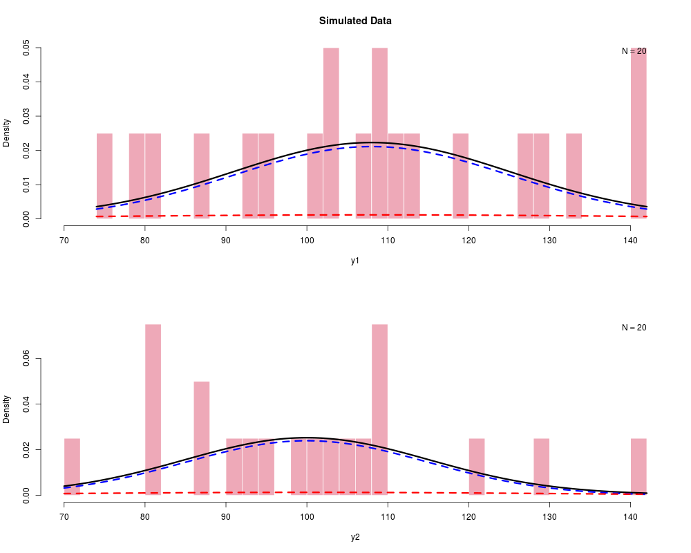
# 1. Generate idealised data set:
proData <- makeData(mu1=108, sd1=17, mu2=100, sd2=15, nPerGrp=20, 
                         pcntOut=10, sdOutMult=2.0, rnd.seed=NULL)

# 2. Generate credible parameter values from the idealised data:
proMCMC <- BESTmcmc(proData$y1, proData$y2, numSavedSteps=2000)  

# 3. Compute the prospective power for planned sample sizes:
# We'll  do just 5 simulations to show it works; should be several hundred.
N1plan <- N2plan <- 50
powerPro <- BESTpower(proMCMC, N1=N1plan, N2=N2plan,
               ROPEm=c(-1.5,1.5), ROPEsd=c(-2,2), ROPEeff=c(-0.5,0.5), 
               maxHDIWm=15.0, maxHDIWsd=10.0, maxHDIWeff=1.0, nRep=5)
powerPro

Results


R version 3.3.1 (2016-06-21) -- "Bug in Your Hair"
Copyright (C) 2016 The R Foundation for Statistical Computing
Platform: x86_64-pc-linux-gnu (64-bit)

R is free software and comes with ABSOLUTELY NO WARRANTY.
You are welcome to redistribute it under certain conditions.
Type 'license()' or 'licence()' for distribution details.

R is a collaborative project with many contributors.
Type 'contributors()' for more information and
'citation()' on how to cite R or R packages in publications.

Type 'demo()' for some demos, 'help()' for on-line help, or
'help.start()' for an HTML browser interface to help.
Type 'q()' to quit R.

> library(BEST)
> png(filename="/home/ddbj/snapshot/RGM3/R_CC/result/BEST/BESTpower.Rd_%03d_medium.png", width=480, height=480)
> ### Name: BESTpower
> ### Title: Estimating statistical power
> ### Aliases: BESTpower
> 
> ### ** Examples
> 
> 
> ## For retrospective power analysis, see the example in BEST-package.
> 
> # 1. Generate idealised data set:
> proData <- makeData(mu1=108, sd1=17, mu2=100, sd2=15, nPerGrp=20, 
+                          pcntOut=10, sdOutMult=2.0, rnd.seed=NULL)
> ## No test: 
> # 2. Generate credible parameter values from the idealised data:
> proMCMC <- BESTmcmc(proData$y1, proData$y2, numSavedSteps=2000)  

Processing function input....... 

Done. 
 
Beginning parallel processing using 3 cores. Console output will be suppressed.

Parallel processing completed.

MCMC took 0.04 minutes.
> 
> # 3. Compute the prospective power for planned sample sizes:
> # We'll  do just 5 simulations to show it works; should be several hundred.
> N1plan <- N2plan <- 50
> powerPro <- BESTpower(proMCMC, N1=N1plan, N2=N2plan,
+                ROPEm=c(-1.5,1.5), ROPEsd=c(-2,2), ROPEeff=c(-0.5,0.5), 
+                maxHDIWm=15.0, maxHDIWsd=10.0, maxHDIWeff=1.0, nRep=5)

:::::::::::::::::::::::::::::::::::::::::::::::::::::::::::::::
Power computation: Simulated Experiment 1 of 5 :


Processing function input....... 

Done. 
 
Beginning parallel processing using 3 cores. Console output will be suppressed.

Parallel processing completed.

MCMC took 0.085 minutes.

After 1 Simulated Experiments, Posterior Probability
         of meeting each criterion is (mean and 95% CrI):
                      mean CrIlo CrIhi
  mean:   HDI > ROPE 0.333 0.000 0.776
  mean:   HDI < ROPE 0.333 0.000 0.776
  mean:  HDI in ROPE 0.333 0.000 0.776
  mean: HDI width ok 0.333 0.000 0.776
    sd:   HDI > ROPE 0.333 0.000 0.776
    sd:   HDI < ROPE 0.333 0.000 0.776
    sd:  HDI in ROPE 0.333 0.000 0.776
    sd: HDI width ok 0.333 0.000 0.776
effect:   HDI > ROPE 0.333 0.000 0.776
effect:   HDI < ROPE 0.333 0.000 0.776
effect:  HDI in ROPE 0.333 0.000 0.776
effect: HDI width ok 0.667 0.224 1.000

:::::::::::::::::::::::::::::::::::::::::::::::::::::::::::::::
Power computation: Simulated Experiment 2 of 5 :


Processing function input....... 

Done. 
 
Beginning parallel processing using 3 cores. Console output will be suppressed.

Parallel processing completed.

MCMC took 0.096 minutes.

After 2 Simulated Experiments, Posterior Probability
         of meeting each criterion is (mean and 95% CrI):
                     mean CrIlo CrIhi
  mean:   HDI > ROPE 0.25 0.000 0.632
  mean:   HDI < ROPE 0.25 0.000 0.632
  mean:  HDI in ROPE 0.25 0.000 0.632
  mean: HDI width ok 0.25 0.000 0.632
    sd:   HDI > ROPE 0.25 0.000 0.632
    sd:   HDI < ROPE 0.25 0.000 0.632
    sd:  HDI in ROPE 0.25 0.000 0.632
    sd: HDI width ok 0.25 0.000 0.632
effect:   HDI > ROPE 0.25 0.000 0.632
effect:   HDI < ROPE 0.25 0.000 0.632
effect:  HDI in ROPE 0.25 0.000 0.632
effect: HDI width ok 0.75 0.368 1.000

:::::::::::::::::::::::::::::::::::::::::::::::::::::::::::::::
Power computation: Simulated Experiment 3 of 5 :


Processing function input....... 

Done. 
 
Beginning parallel processing using 3 cores. Console output will be suppressed.

Parallel processing completed.

MCMC took 0.122 minutes.

After 3 Simulated Experiments, Posterior Probability
         of meeting each criterion is (mean and 95% CrI):
                     mean CrIlo CrIhi
  mean:   HDI > ROPE  0.2 0.000 0.527
  mean:   HDI < ROPE  0.2 0.000 0.527
  mean:  HDI in ROPE  0.2 0.000 0.527
  mean: HDI width ok  0.2 0.000 0.527
    sd:   HDI > ROPE  0.2 0.000 0.527
    sd:   HDI < ROPE  0.2 0.000 0.527
    sd:  HDI in ROPE  0.2 0.000 0.527
    sd: HDI width ok  0.2 0.000 0.527
effect:   HDI > ROPE  0.2 0.000 0.527
effect:   HDI < ROPE  0.2 0.000 0.527
effect:  HDI in ROPE  0.2 0.000 0.527
effect: HDI width ok  0.8 0.473 1.000

:::::::::::::::::::::::::::::::::::::::::::::::::::::::::::::::
Power computation: Simulated Experiment 4 of 5 :


Processing function input....... 

Done. 
 
Beginning parallel processing using 3 cores. Console output will be suppressed.

Parallel processing completed.

MCMC took 0.105 minutes.

After 4 Simulated Experiments, Posterior Probability
         of meeting each criterion is (mean and 95% CrI):
                      mean CrIlo CrIhi
  mean:   HDI > ROPE 0.167 0.000 0.451
  mean:   HDI < ROPE 0.167 0.000 0.451
  mean:  HDI in ROPE 0.167 0.000 0.451
  mean: HDI width ok 0.167 0.000 0.451
    sd:   HDI > ROPE 0.167 0.000 0.451
    sd:   HDI < ROPE 0.167 0.000 0.451
    sd:  HDI in ROPE 0.167 0.000 0.451
    sd: HDI width ok 0.167 0.000 0.451
effect:   HDI > ROPE 0.167 0.000 0.451
effect:   HDI < ROPE 0.167 0.000 0.451
effect:  HDI in ROPE 0.167 0.000 0.451
effect: HDI width ok 0.833 0.549 1.000

:::::::::::::::::::::::::::::::::::::::::::::::::::::::::::::::
Power computation: Simulated Experiment 5 of 5 :


Processing function input....... 

Done. 
 
Beginning parallel processing using 3 cores. Console output will be suppressed.

Parallel processing completed.

MCMC took 0.096 minutes.

After 5 Simulated Experiments, Posterior Probability
         of meeting each criterion is (mean and 95% CrI):
                      mean CrIlo CrIhi
  mean:   HDI > ROPE 0.143 0.000 0.393
  mean:   HDI < ROPE 0.143 0.000 0.393
  mean:  HDI in ROPE 0.143 0.000 0.393
  mean: HDI width ok 0.143 0.000 0.393
    sd:   HDI > ROPE 0.143 0.000 0.393
    sd:   HDI < ROPE 0.143 0.000 0.393
    sd:  HDI in ROPE 0.143 0.000 0.393
    sd: HDI width ok 0.143 0.000 0.393
effect:   HDI > ROPE 0.143 0.000 0.393
effect:   HDI < ROPE 0.143 0.000 0.393
effect:  HDI in ROPE 0.286 0.018 0.591
effect: HDI width ok 0.857 0.607 1.000
> powerPro
                          mean        CrIlo     CrIhi
  mean:   HDI > ROPE 0.1428571 1.057369e-09 0.3930378
  mean:   HDI < ROPE 0.1428571 1.057369e-09 0.3930378
  mean:  HDI in ROPE 0.1428571 1.057369e-09 0.3930378
  mean: HDI width ok 0.1428571 1.057369e-09 0.3930378
    sd:   HDI > ROPE 0.1428571 1.057369e-09 0.3930378
    sd:   HDI < ROPE 0.1428571 1.057369e-09 0.3930378
    sd:  HDI in ROPE 0.1428571 1.057369e-09 0.3930378
    sd: HDI width ok 0.1428571 1.057369e-09 0.3930378
effect:   HDI > ROPE 0.1428571 1.057369e-09 0.3930378
effect:   HDI < ROPE 0.1428571 1.057369e-09 0.3930378
effect:  HDI in ROPE 0.2857143 1.782673e-02 0.5906173
effect: HDI width ok 0.8571429 6.069622e-01 1.0000000
> ## End(No test)
> 
> 
> 
> 
> 
> dev.off()
null device 
          1 
>