Highest Density Interval

Description

Calculate the highest density interval (HDI) for a given probability mass, see Details. The function is generic, with methods for a range of input objects.

Usage

hdi(object, credMass = 0.95, ...)

## Default S3 method:
hdi(object, credMass = 0.95, ...)

## S3 method for class 'function'
hdi(object, credMass = 0.95, tol, ...)

## S3 method for class 'matrix'
hdi(object, credMass = 0.95, ...)

## S3 method for class 'data.frame'
hdi(object, credMass = 0.95, ...)

## S3 method for class 'density'
hdi(object, credMass = 0.95, allowSplit=FALSE, ...)

## S3 method for class 'mcmc.list'
hdi(object, credMass = 0.95, ...)

Arguments

Details

The HDI is the interval which contains the required mass such that all points within the interval have a higher probability density than points outside the interval. When applied to a posterior probability density, it is often known as the Highest Posterior Density (HPD).

In contrast, a symmetric density interval defined by (eg.) the 10% and 90% quantiles may include values with lower probability than those excluded.

For a unimodal distribution, the HDI is the narrowest interval containing the specified mass, and the hdi function actually returns the narrowest interval. This does not always work properly for multimodel densities, where the HDI may be discontinuous (the horizontal black line in the Figure below). The single interval returned by hdi (the blue line) may incorrectly include values between the modes with low probability density. The density method with allowSplit = TRUE gives separate limits for discontinuous HDIs.

The default method expects a vector representing draws from the target distribution, such as is produced by an MCMC process. Missing values are silently ignored; if the vector has no non-missing values, NAs are returned.

The matrix and data frame methods expect an object with vectors of the above type for each parameter in columns. The result is a matrix with parameters in columns, and rows with the upper and lower limits of the HDI.

The mcmc.list method expects an object of type mcmc.list as defined in package coda.

None of the above use interpolation: the values returned correspond to specific values in the data object. Results thus depend on the random draws, and will be unstable if few values are provided. For a 95% HDI, 10,000 independent draws are recommended; a smaller number will be adequate for a 80% HDI, many more for a 99% HDI.

The function method requires the name for the inverse cumulative density function (ICDF) of the distribution; standard R functions for this have a q- prefix, eg. qbeta. Arguments required by the ICDF must be specified by their (abbreviated) names; see the examples.

Value

a vector of length 2 or a 2-row matrix with the lower and upper limits of the HDI, with an attribute "credMass".

The density method with allowSplit = TRUE produces a matrix with a row for each component of a discontinuous HDI and columns for begin and end. It has an additional attribute "height" giving the probability density at the limits of the HDI.

Author(s)

Mike Meredith. Code for hdi.function based on hpd by Greg Snow, corrected by John Kruschke.

References

Kruschke, J. K. 2011. Doing Bayesian data analysis: a tutorial with R and BUGS. Elsevier, Amsterdam, section 3.3.5.

Examples

# for a vector:
tst <- rgamma(1e5, 2.5, 2)
hdi(tst)
hdi(tst, credMass=0.8)
# For comparison, the symmetrical 80% CrI:
quantile(tst, c(0.1,0.9))

# Now a data frame:
tst <- data.frame(mu = rnorm(1e4, 4, 1), sigma = rlnorm(1e4))
hdi(tst, 0.8)
apply(tst, 2, quantile, c(0.1,0.9))

# For a function:
hdi(qgamma, 0.8, shape=2.5, rate=2)
# and the symmetrical 80% CrI:
qgamma(c(0.1, 0.9), 2.5, 2)

# A severely bimodal distribution:
tst2 <- c(rnorm(1e5), rnorm(5e4, 7))
hist(tst2, freq=FALSE)
(hdiMC <- hdi(tst2))
segments(hdiMC[1], 0, hdiMC[2], 0, lwd=3, col='red')
# This is a valid 95% CrI, but not a Highest Density Interval

dens2 <- density(tst2)
lines(dens2, lwd=2, col='blue')
(hdiD1 <- hdi(dens2))  # default allowSplit = FALSE; note the warning
segments(hdiD1[1], 0.01, hdiD1[2], 0.01, lty=3, col='blue')
# This is a valid 95% CrI, but not an HDI
(hdiD2 <- hdi(dens2, allowSplit=TRUE))
(ht <- attr(hdiD2, "height"))
segments(hdiD2[, 1], ht, hdiD2[, 2], ht, lwd=3, col='blue')
# This is the correct 95% HDI.

Results

R version 3.3.1 (2016-06-21) -- "Bug in Your Hair"
Copyright (C) 2016 The R Foundation for Statistical Computing
Platform: x86_64-pc-linux-gnu (64-bit)

R is free software and comes with ABSOLUTELY NO WARRANTY.
You are welcome to redistribute it under certain conditions.
Type 'license()' or 'licence()' for distribution details.

R is a collaborative project with many contributors.
Type 'contributors()' for more information and
'citation()' on how to cite R or R packages in publications.

Type 'demo()' for some demos, 'help()' for on-line help, or
'help.start()' for an HTML browser interface to help.
Type 'q()' to quit R.

> library(BEST)
> png(filename="/home/ddbj/snapshot/RGM3/R_CC/result/BEST/hdi.Rd_%03d_medium.png", width=480, height=480)
> ### Name: hdi
> ### Title: Highest Density Interval
> ### Aliases: hdi hdi.default hdi.function hdi.matrix hdi.data.frame
> ###   hdi.density hdi.mcmc.list
> ### Keywords: methods htest
> 
> ### ** Examples
> 
> # for a vector:
> tst <- rgamma(1e5, 2.5, 2)
> hdi(tst)
     lower      upper 
0.09183344 2.82428024 
attr(,"credMass")
[1] 0.95
> hdi(tst, credMass=0.8)
   lower    upper 
0.194361 1.903230 
attr(,"credMass")
[1] 0.8
> # For comparison, the symmetrical 80% CrI:
> quantile(tst, c(0.1,0.9))
     10%      90% 
0.403489 2.310669 
> 
> # Now a data frame:
> tst <- data.frame(mu = rnorm(1e4, 4, 1), sigma = rlnorm(1e4))
> hdi(tst, 0.8)
            mu      sigma
lower 2.728598 0.05449496
upper 5.238388 2.34642114
attr(,"credMass")
[1] 0.8
> apply(tst, 2, quantile, c(0.1,0.9))
          mu     sigma
10% 2.728571 0.2833976
90% 5.238360 3.5011073
> 
> # For a function:
> hdi(qgamma, 0.8, shape=2.5, rate=2)
    lower     upper 
0.1947158 1.9053925 
attr(,"credMass")
[1] 0.8
> # and the symmetrical 80% CrI:
> qgamma(c(0.1, 0.9), 2.5, 2)
[1] 0.402577 2.309089
> 
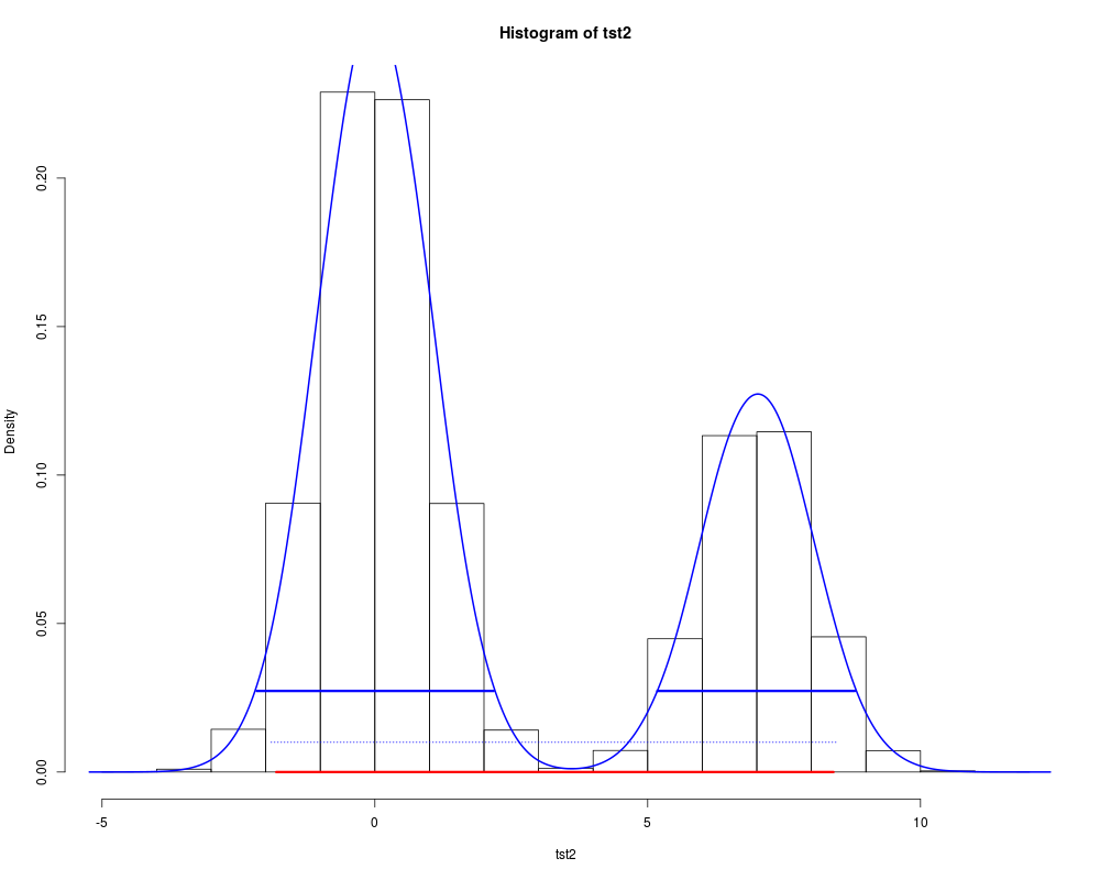
> # A severely bimodal distribution:
> tst2 <- c(rnorm(1e5), rnorm(5e4, 7))
> hist(tst2, freq=FALSE)
> (hdiMC <- hdi(tst2))
    lower     upper 
-1.830860  8.375436 
attr(,"credMass")
[1] 0.95
> segments(hdiMC[1], 0, hdiMC[2], 0, lwd=3, col='red')
> # This is a valid 95% CrI, but not a Highest Density Interval
> 
> dens2 <- density(tst2)
> lines(dens2, lwd=2, col='blue')
> (hdiD1 <- hdi(dens2))  # default allowSplit = FALSE; note the warning
    lower     upper 
-1.931874  8.437095 
attr(,"credMass")
[1] 0.95
attr(,"height")
[1] 0.02747916
Warning message:
In hdi.density(dens2) : The HDI is discontinuous but allowSplit = FALSE;
    the result is a valid CrI but not HDI.
> segments(hdiD1[1], 0.01, hdiD1[2], 0.01, lty=3, col='blue')
> # This is a valid 95% CrI, but not an HDI
> (hdiD2 <- hdi(dens2, allowSplit=TRUE))
         begin      end
[1,] -2.197291 2.190942
[2,]  5.199004 8.808680
attr(,"credMass")
[1] 0.95
attr(,"height")
[1] 0.02747916
> (ht <- attr(hdiD2, "height"))
[1] 0.02747916
> segments(hdiD2[, 1], ht, hdiD2[, 2], ht, lwd=3, col='blue')
> # This is the correct 95% HDI.
> 
> 
> 
> 
> 
> dev.off()
null device 
          1 
>