R Graphical Manual

Browse All

Last data update: 2014.03.03

R: Graphic display of a posterior probability distribution

plotPost

R Documentation

Graphic display of a posterior probability distribution

Description

Plot the posterior probability distribution for a single parameter from a vector of samples, typically from an MCMC process, with appropriate summary statistics.

Usage

plotPost(paramSampleVec, credMass = 0.95, compVal = NULL, ROPE = NULL,
  HDItextPlace = 0.7, showMode = FALSE, showCurve = FALSE, ...)

Arguments

`paramSampleVec`	A vector of samples drawn from the target distribution.
`credMass`	the probability mass to include in credible intervals, or NULL to suppress plotting of credible intervals.
`compVal`	a value for comparison with those plotted.
`ROPE`	a two element vector, such as `c(-1, 1)`, specifying the limits of the Region Of Practical Equivalence.
`HDItextPlace`	a value in [0,1] that controls the horizontal position of the labels at the ends of the HDI bar.
`showMode`	logical: if TRUE, the mode is displayed instead of the mean.
`showCurve`	logical: if TRUE, the posterior density will be represented by a kernel density function instead of a histogram.
`...`	graphical parameters and the `breaks` parameter for the histogram.

Details

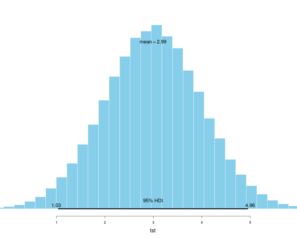
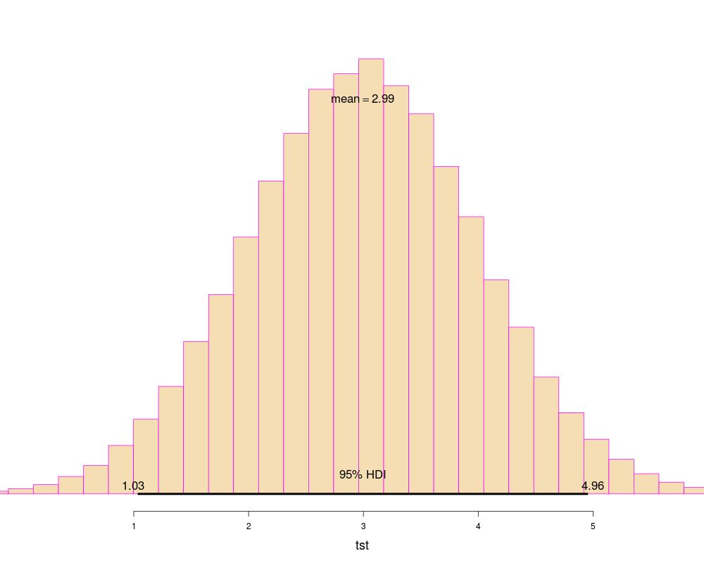
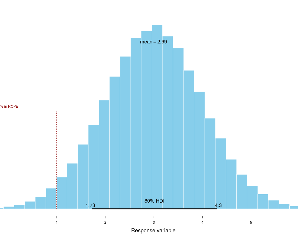
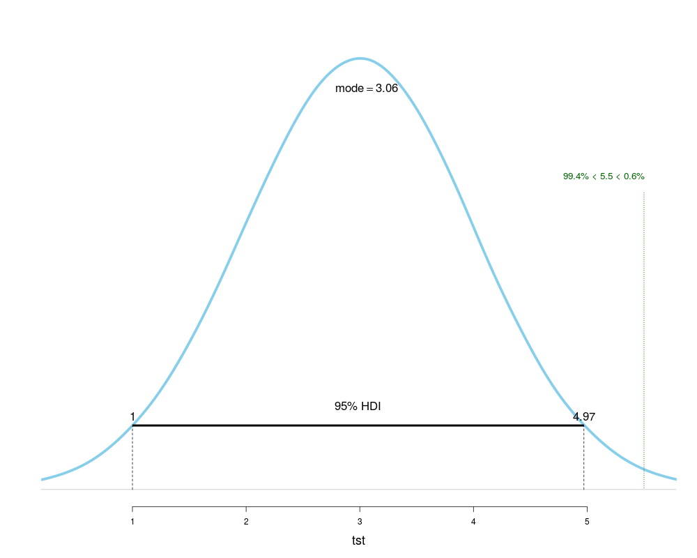
The data are plotted either as a histogram (above) or, if showCurve = TRUE, as a fitted kernel density curve (below). Either the mean or the mode of the distribution is displayed, depending on the parameter showMode. The Highest Density Interval (HDI) is shown as a horizontal bar, with labels for the ends of the interval.

If values for a ROPE are supplied, these are shown as dark red vertical dashed lines, together with the percentage of probability mass within the ROPE. If a comparison value (compVal) is supplied, this is shown as a vertical green dotted line, together with the probability mass below and above this value.

Value

Returns an object of class histogram invisibly. Used for its plotting side-effect.

Author(s)

John Kruschke, modified by Mike Meredith

Examples

# Generate some data
tst <- rnorm(1e5, 3, 1)
plotPost(tst)
plotPost(tst, col='wheat', border='magenta')
plotPost(tst, credMass=0.8, ROPE=c(-1,1), xlab="Response variable")
plotPost(tst, showMode=TRUE, showCurve=TRUE, compVal=5.5)

# For integers:
tst <- rpois(1e5, 12)
plotPost(tst)

# A severely bimodal distribution:
tst2 <- c(rnorm(1e5), rnorm(5e4, 7))
plotPost(tst2)                  # A valid 95% CrI, but not HDI
plotPost(tst2, showCurve=TRUE)  # Correct 95% HDI

Results


R version 3.3.1 (2016-06-21) -- "Bug in Your Hair"
Copyright (C) 2016 The R Foundation for Statistical Computing
Platform: x86_64-pc-linux-gnu (64-bit)

R is free software and comes with ABSOLUTELY NO WARRANTY.
You are welcome to redistribute it under certain conditions.
Type 'license()' or 'licence()' for distribution details.

R is a collaborative project with many contributors.
Type 'contributors()' for more information and
'citation()' on how to cite R or R packages in publications.

Type 'demo()' for some demos, 'help()' for on-line help, or
'help.start()' for an HTML browser interface to help.
Type 'q()' to quit R.

> library(BEST)
> png(filename="/home/ddbj/snapshot/RGM3/R_CC/result/BEST/plotPost.Rd_%03d_medium.png", width=480, height=480)
> ### Name: plotPost
> ### Title: Graphic display of a posterior probability distribution
> ### Aliases: plotPost
> ### Keywords: hplot
> 
> ### ** Examples
> 
> # Generate some data
> tst <- rnorm(1e5, 3, 1)
> plotPost(tst)
> plotPost(tst, col='wheat', border='magenta')
> plotPost(tst, credMass=0.8, ROPE=c(-1,1), xlab="Response variable")
> plotPost(tst, showMode=TRUE, showCurve=TRUE, compVal=5.5)
> 
> # For integers:
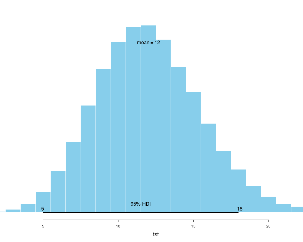
> tst <- rpois(1e5, 12)
> plotPost(tst)
> 
> # A severely bimodal distribution:
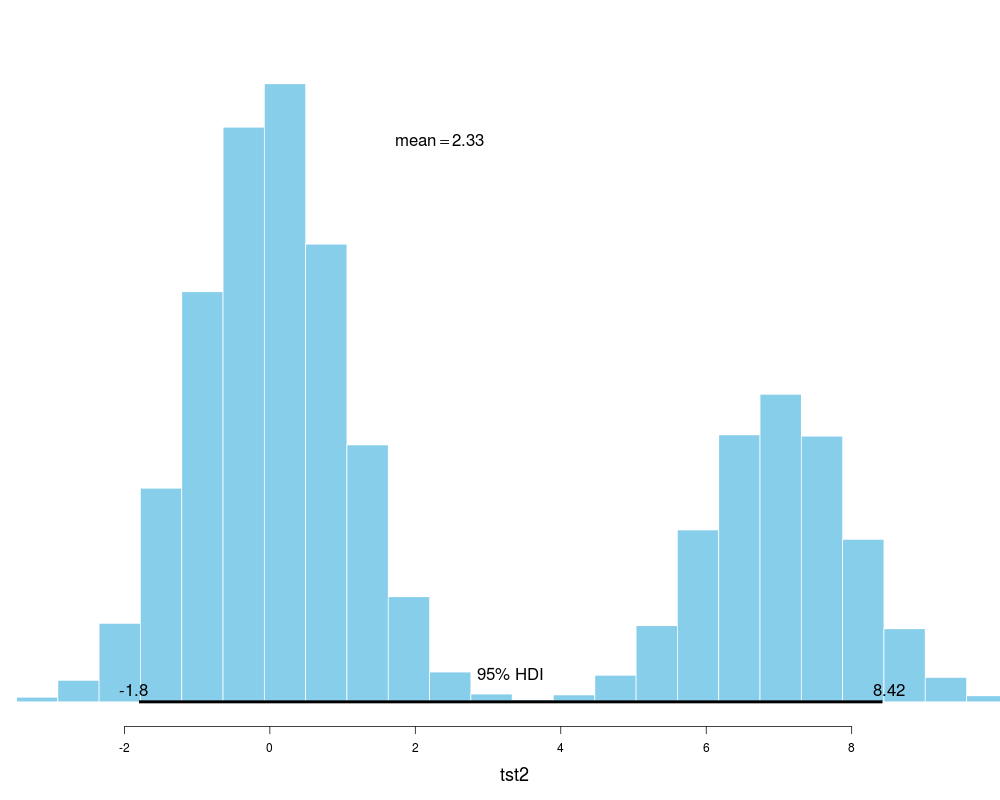
> tst2 <- c(rnorm(1e5), rnorm(5e4, 7))
> plotPost(tst2)                  # A valid 95% CrI, but not HDI
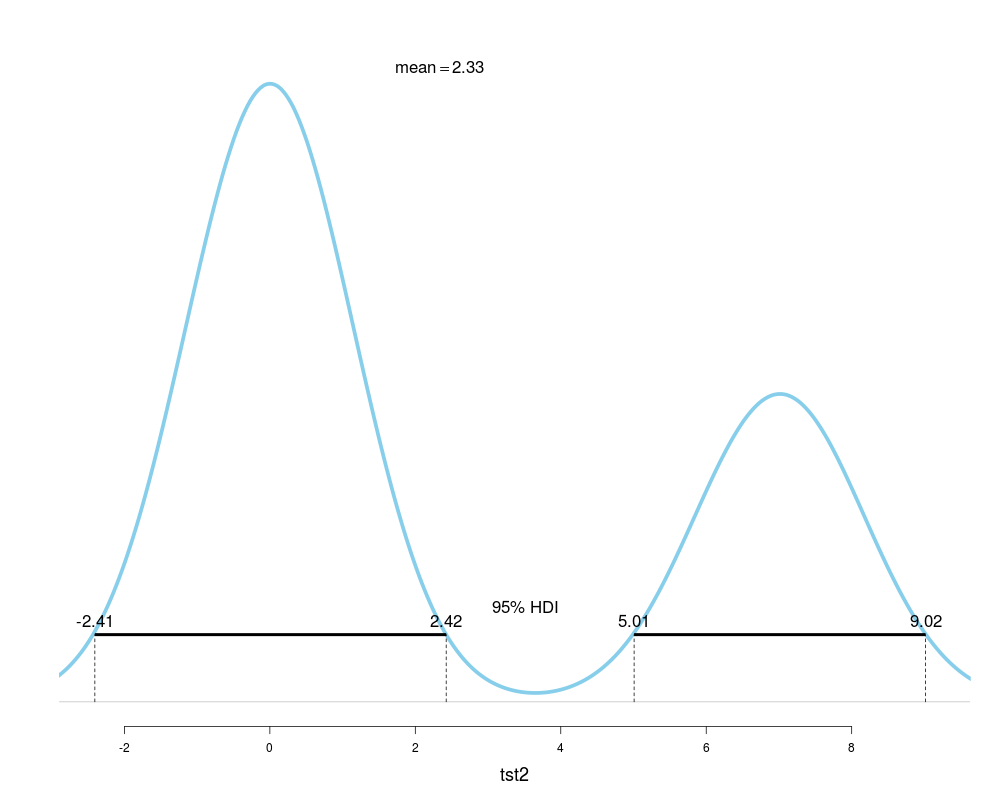
> plotPost(tst2, showCurve=TRUE)  # Correct 95% HDI
> 
> 
> 
> 
> 
> 
> dev.off()
null device 
          1 
>