Supported by Dr. Osamu Ogasawara and  . . |
|
Last data update: 2014.03.03 |
Graphical AnovaDescriptionDots plot displaying the deviations of factor levels from the mean showing the residuals as reference distribution. Usage
    anovaPlot(obj, stacked = TRUE, base = TRUE, axes = TRUE,
    faclab = TRUE, labels = FALSE, cex = par("cex"),
    cex.lab = par("cex.lab"), ...)
Arguments
DetailsDots plot are displayed for the scaled deviations of factor levels from
the grand mean and the distribution of the residuals is shown at the bottom
of the plot for graphical comparison. The scaled factor for the factor
deviations is sqrt(n / k), where k and n
are the factor and residuals degrees of freedom reported by ValueThe function is called for graphical display of factor levels mean and residuals as reference distribution. An invisible list with the actual (x,y) coordinates used for each of the factors and residuals. warningThe function identifies as an interaction factor any factor with the colon character ":" in its name. Factors like "I(A:B)" will give you problems. NoteThe anova plot presented here is thought for graphical comparison of factor effects in one-layer balanced designed experiments. The function is not prepared for general situations. However, representation of some simple split-plot experiments is possible. Author(s)Ernesto Barrios ReferencesBox G. E. P. (2000). Box on Quality. Edited by G. C. Tiao et al. New York: Wiley. Box G. E. P, Hunter, J. S. and Hunter, W. C. (2005). Statistics for Experimenters II. New York: Wiley. See Also
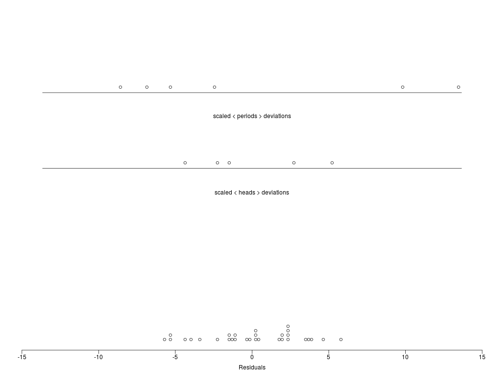
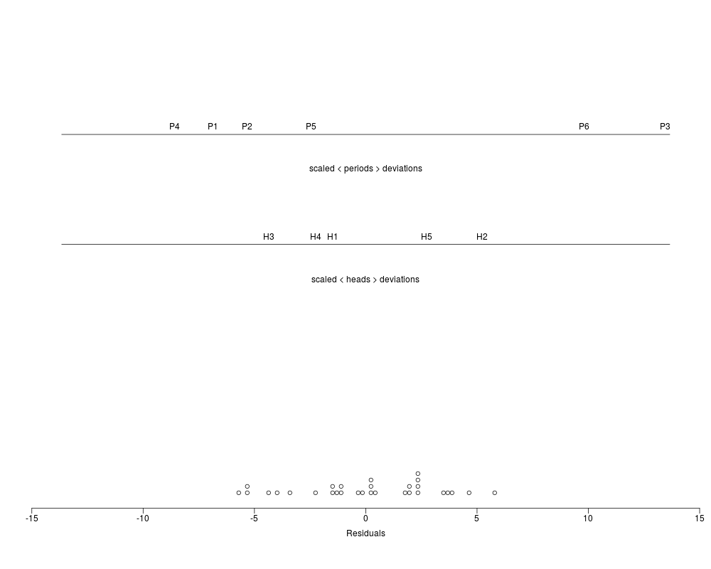
Exampleslibrary(BHH2) data(heads.data) heads.data$periods <- factor(heads.data$periods) heads.data$heads <- factor(heads.data$heads) heads.aov <- aov(resp~periods+heads,data=heads.data) anovaPlot(heads.aov) anovaPlot(heads.aov,labels=TRUE,faclab=TRUE) Results
R version 3.3.1 (2016-06-21) -- "Bug in Your Hair"
Copyright (C) 2016 The R Foundation for Statistical Computing
Platform: x86_64-pc-linux-gnu (64-bit)

R is free software and comes with ABSOLUTELY NO WARRANTY.
You are welcome to redistribute it under certain conditions.
Type 'license()' or 'licence()' for distribution details.

R is a collaborative project with many contributors.
Type 'contributors()' for more information and
'citation()' on how to cite R or R packages in publications.

Type 'demo()' for some demos, 'help()' for on-line help, or
'help.start()' for an HTML browser interface to help.
Type 'q()' to quit R.

> library(BHH2)
> png(filename="/home/ddbj/snapshot/RGM3/R_CC/result/BHH2/anovaPlot.Rd_%03d_medium.png", width=480, height=480)
> ### Name: anovaPlot
> ### Title: Graphical Anova
> ### Aliases: anovaPlot
> ### Keywords: design hplot regression
>
> ### ** Examples
>
> library(BHH2)
> data(heads.data)
> heads.data$periods <- factor(heads.data$periods)
> heads.data$heads <- factor(heads.data$heads)
>
> heads.aov <- aov(resp~periods+heads,data=heads.data)
> anovaPlot(heads.aov)
>
> anovaPlot(heads.aov,labels=TRUE,faclab=TRUE)
>
>
>
>
>
>
> dev.off()
null device
          1
>
|