Last data update: 2014.03.03
R: Empirical Distribution Function and Quantiles
BIFIE.ecdf R Documentation
Empirical Distribution Function and Quantiles
Description
Computes an empirical distribution function (and quantiles).
If only some quantiles should
be calculated, then an appropriate vector of breaks (which are quantiles)
must be specified.
Statistical inference is not conducted for this method.
Usage
BIFIE.ecdf( BIFIEobj, vars , breaks=NULL, quanttype=1, group=NULL , group_values=NULL )

## S3 method for class 'BIFIE.ecdf'
summary(object,digits=4,...)
Arguments
BIFIEobj
Object of class BIFIEdata
vars
Vector of variables for which statistics should be computed.
breaks
Optional vector of breaks. Otherwise, it will be automatically defined.
quanttype
Type of calculation for quantiles. In case of quanttype=1,
a linear interpolation is used while for quanttype=2 it is not.
group
Optional grouping variable
group_values
Optional vector of grouping values. This can be omitted and grouping
values will be determined automatically.
object
Object of class BIFIE.ecdf
digits
Number of digits for rounding output
...
Further arguments to be passed
Value
A list with following entries
ecdf
Data frame with probabilities and the empirical
distribution function (See Examples).
output
More extensive output
...
More values
See Also
Hmisc::wtd.ecdf,
Hmisc::wtd.quantile
Examples
#############################################################################
# EXAMPLE 1: Imputed TIMSS dataset
#############################################################################
data(data.timss1)
data(data.timssrep)
# create BIFIE.dat object
bifieobj <- BIFIE.data( data.list=data.timss1 , wgt= data.timss1[[1]]$TOTWGT ,
wgtrep=data.timssrep[, -1 ] )
# ecdf
vars <- c( "ASMMAT" , "books")
group <- "female" ; group_values <- 0:1
# quantile type 1
res1 <- BIFIE.ecdf( bifieobj , vars = vars , group=group )
summary(res1)
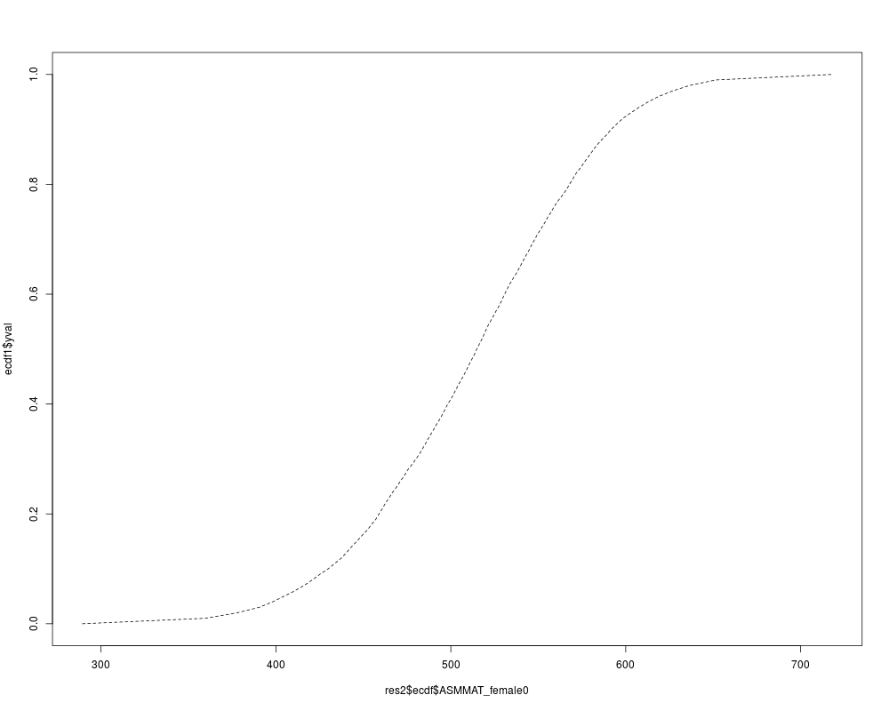
res2 <- BIFIE.ecdf( bifieobj , vars = vars , group=group , quanttype=2)
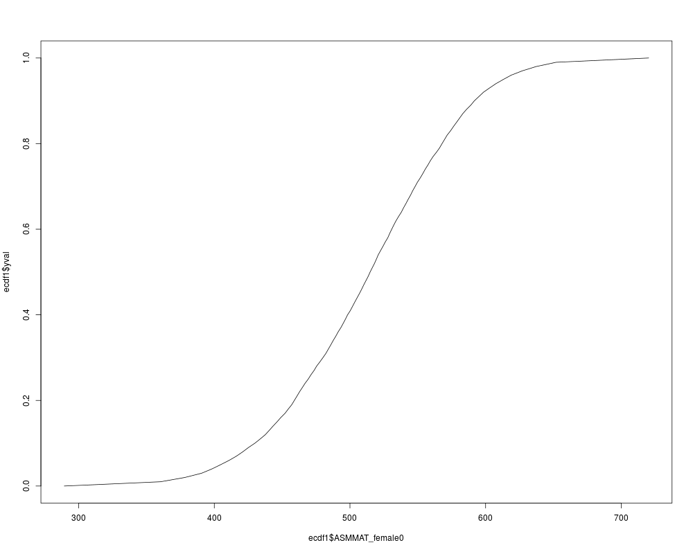
# plot distribution function
ecdf1 <- res1$ecdf
plot( ecdf1$ASMMAT_female0 , ecdf1$yval , type="l")
plot( res2$ecdf$ASMMAT_female0 , ecdf1$yval , type="l" , lty=2)
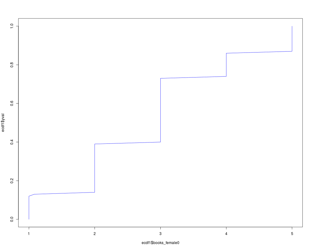
plot( ecdf1$books_female0 , ecdf1$yval , type="l" , col="blue")
Results
R version 3.3.1 (2016-06-21) -- "Bug in Your Hair"
Copyright (C) 2016 The R Foundation for Statistical Computing
Platform: x86_64-pc-linux-gnu (64-bit)

R is free software and comes with ABSOLUTELY NO WARRANTY.
You are welcome to redistribute it under certain conditions.
Type 'license()' or 'licence()' for distribution details.

R is a collaborative project with many contributors.
Type 'contributors()' for more information and
'citation()' on how to cite R or R packages in publications.

Type 'demo()' for some demos, 'help()' for on-line help, or
'help.start()' for an HTML browser interface to help.
Type 'q()' to quit R.

> library(BIFIEsurvey)
|-----------------------------------------------------------------
| BIFIEsurvey 1.9.4-0 (2016-06-01)
| http://www.bifie.at
|-----------------------------------------------------------------

> png(filename="/home/ddbj/snapshot/RGM3/R_CC/result/BIFIEsurvey/BIFIE.ecdf.Rd_%03d_medium.png", width=480, height=480)
> ### Name: BIFIE.ecdf
> ### Title: Empirical Distribution Function and Quantiles
> ### Aliases: BIFIE.ecdf summary.BIFIE.ecdf
> ### Keywords: Empirical distribution function Quantiles summary
>
> ### ** Examples
>
> #############################################################################
> # EXAMPLE 1: Imputed TIMSS dataset
> #############################################################################
>
> data(data.timss1)
> data(data.timssrep)
>
> # create BIFIE.dat object
> bifieobj <- BIFIE.data( data.list=data.timss1 , wgt=  data.timss1[[1]]$TOTWGT ,
+            wgtrep=data.timssrep[, -1 ] )
+++ Generate BIFIE.data object
|*****|
|-----|
>
> # ecdf
> vars <- c( "ASMMAT" , "books")
> group <- "female" ; group_values <- 0:1
> # quantile type 1
> res1 <- BIFIE.ecdf( bifieobj ,  vars = vars , group=group )
|*****|
> summary(res1)
------------------------------------------------------------
BIFIEsurvey 1.9.4-0 (2016-06-01)
Function 'BIFIE.ecdf'

Call:
BIFIE.ecdf(BIFIEobj = bifieobj, vars = vars, group = group)

Date of Analysis: 2016-07-04 14:24:51
Time difference of 0.01668668 secs
Computation time: 0.01668668

Multiply imputed dataset

Number of persons = 4668
Number of imputed datasets = 5
Number of Jackknife zones per dataset = 0
Fay factor = 1

Empirical Distribution Function
    yval ASMMAT_female0 ASMMAT_female1 books_female0 books_female1
1   0.00       289.4060       289.2616        1.0000        1.0000
2   0.01       360.4102       350.5463        1.0000        1.0000
3   0.02       378.2956       370.2925        1.0000        1.0000
4   0.03       390.7284       382.2644        1.0000        1.0000
5   0.04       398.2713       391.3413        1.0000        1.0000
6   0.05       404.7193       399.0253        1.0000        1.0000
7   0.06       410.9382       404.2058        1.0000        1.0000
8   0.07       416.3854       409.1407        1.0000        2.0000
9   0.08       420.9947       413.9343        1.0000        2.0000
10  0.09       425.1791       418.1969        1.0000        2.0000
11  0.10       429.8868       422.6586        1.0000        2.0000
12  0.11       433.8429       425.8044        1.0000        2.0000
13  0.12       437.6019       428.9276        1.0000        2.0000
14  0.13       440.4902       432.0660        1.0824        2.0000
15  0.14       443.2934       434.9671        2.0000        2.0000
16  0.15       446.2621       437.8459        2.0000        2.0000
17  0.16       449.0259       441.0204        2.0000        2.0000
18  0.17       452.1626       443.5597        2.0000        2.0000
19  0.18       454.5535       446.1485        2.0000        2.0000
20  0.19       457.0869       448.4907        2.0000        2.0000
21  0.20       458.9986       450.8571        2.0000        2.0000
22  0.21       460.9323       453.0013        2.0000        2.0000
23  0.22       462.7966       455.4279        2.0000        2.0000
24  0.23       464.8803       458.1117        2.0000        2.0000
25  0.24       466.9136       460.2872        2.0000        2.0000
26  0.25       469.2726       462.6059        2.0000        2.0000
27  0.26       471.2657       464.5962        2.0000        2.0000
28  0.27       473.5467       466.6757        2.0000        2.0000
29  0.28       475.4000       468.6870        2.0000        2.0000
30  0.29       477.8102       470.4226        2.0000        2.0000
31  0.30       480.0956       472.2576        2.0000        2.0000
32  0.31       482.2891       474.2782        2.0000        2.0000
33  0.32       484.0860       475.9431        2.0000        2.0000
34  0.33       485.9087       477.6245        2.0000        2.4603
35  0.34       487.6431       479.6084        2.0000        3.0000
36  0.35       489.5604       481.2537        2.0000        3.0000
37  0.36       491.2799       483.2301        2.0000        3.0000
38  0.37       493.2986       484.8385        2.0000        3.0000
39  0.38       495.0179       486.7814        2.0000        3.0000
40  0.39       496.6917       488.4322        2.0000        3.0000
41  0.40       498.2431       490.2857        3.0000        3.0000
42  0.41       500.2859       492.0067        3.0000        3.0000
43  0.42       501.9409       493.5864        3.0000        3.0000
44  0.43       503.5877       495.2050        3.0000        3.0000
45  0.44       505.3102       497.0009        3.0000        3.0000
46  0.45       507.0328       498.5194        3.0000        3.0000
47  0.46       508.6513       499.8466        3.0000        3.0000
48  0.47       510.1753       501.5958        3.0000        3.0000
49  0.48       511.8156       503.2402        3.0000        3.0000
50  0.49       513.4574       504.9194        3.0000        3.0000
51  0.50       514.8680       506.4329        3.0000        3.0000
52  0.51       516.4589       507.9330        3.0000        3.0000
53  0.52       518.0709       509.7049        3.0000        3.0000
54  0.53       519.4852       511.5210        3.0000        3.0000
55  0.54       520.8204       512.9131        3.0000        3.0000
56  0.55       522.5602       514.5176        3.0000        3.0000
57  0.56       524.3329       516.1179        3.0000        3.0000
58  0.57       525.9898       517.9863        3.0000        3.0000
59  0.58       527.8937       519.5515        3.0000        3.0000
60  0.59       529.2754       521.1383        3.0000        3.0000
61  0.60       530.7957       522.9874        3.0000        3.0000
62  0.61       532.3495       524.4240        3.0000        3.0000
63  0.62       534.0085       526.0524        3.0000        3.0000
64  0.63       535.8988       527.7227        3.0000        3.0000
65  0.64       537.9137       529.3551        3.0000        3.0000
66  0.65       539.5138       531.0225        3.0000        3.0000
67  0.66       541.2964       532.4859        3.0000        3.0000
68  0.67       542.9439       534.1731        3.0000        3.0000
69  0.68       544.7335       535.5444        3.0000        3.0000
70  0.69       546.2788       537.1540        3.0000        3.0000
71  0.70       548.0536       538.7727        3.0000        3.0000
72  0.71       549.7821       540.3485        3.0000        3.0000
73  0.72       551.8408       541.8885        3.0000        4.0000
74  0.73       553.7181       543.8178        3.0000        4.0000
75  0.74       555.4481       545.5449        4.0000        4.0000
76  0.75       557.4563       547.2582        4.0000        4.0000
77  0.76       559.2689       549.2598        4.0000        4.0000
78  0.77       561.3302       550.8590        4.0000        4.0000
79  0.78       563.8103       552.8609        4.0000        4.0000
80  0.79       566.0606       554.5632        4.0000        4.0000
81  0.80       567.8897       556.6981        4.0000        4.0000
82  0.81       569.7978       559.0376        4.0000        4.0000
83  0.82       571.6767       560.6622        4.0000        4.0000
84  0.83       574.1766       562.9315        4.0000        4.0000
85  0.84       576.3203       565.0438        4.0000        4.0000
86  0.85       578.6383       567.4220        4.0000        4.0000
87  0.86       580.9051       569.8376        4.0000        4.0000
88  0.87       583.1823       572.2332        5.0000        4.0000
89  0.88       585.9448       574.8882        5.0000        4.0000
90  0.89       589.1086       578.0211        5.0000        5.0000
91  0.90       591.7039       580.5636        5.0000        5.0000
92  0.91       595.0740       583.8702        5.0000        5.0000
93  0.92       598.3910       586.9706        5.0000        5.0000
94  0.93       602.9135       589.8593        5.0000        5.0000
95  0.94       607.5578       593.8227        5.0000        5.0000
96  0.95       613.1091       597.9249        5.0000        5.0000
97  0.96       618.9041       603.1582        5.0000        5.0000
98  0.97       627.0231       609.0026        5.0000        5.0000
99  0.98       637.2005       619.0757        5.0000        5.0000
100 0.99       651.9489       629.8061        5.0000        5.0000
101 1.00       720.2110       739.7378        5.0000        5.0000
> res2 <- BIFIE.ecdf( bifieobj ,  vars = vars , group=group , quanttype=2)
|*****|
> # plot distribution function
> ecdf1 <- res1$ecdf
> plot( ecdf1$ASMMAT_female0 , ecdf1$yval , type="l")
> plot( res2$ecdf$ASMMAT_female0 , ecdf1$yval , type="l" , lty=2)
> plot( ecdf1$books_female0 , ecdf1$yval , type="l" , col="blue")
>
>
>
>
>
> dev.off()
null device
          1
>
 .
.