R Graphical Manual

Browse All

Last data update: 2014.03.03

R: Bayesian Model Averaging for linear regression models.

bicreg

R Documentation

Bayesian Model Averaging for linear regression models.

Description

Bayesian Model Averaging accounts for the model uncertainty inherent in the variable selection problem by averaging over the best models in the model class according to approximate posterior model probability.

Usage

bicreg(x, y, wt = rep(1, length(y)), strict = FALSE, OR = 20, 
       maxCol = 31, drop.factor.levels = TRUE, nbest = 150)

Arguments

`x`	a matrix of independent variables
`y`	a vector of values for the dependent variable
`wt`	a vector of weights for regression
`strict`	logical. FALSE returns all models whose posterior model probability is within a factor of 1/OR of that of the best model. TRUE returns a more parsimonious set of models, where any model with a more likely submodel is eliminated.
`OR`	a number specifying the maximum ratio for excluding models in Occam's window
`maxCol`	a number specifying the maximum number of columns in the design matrix (including the intercept) to be kept.
`drop.factor.levels`	logical. Indicates whether factor levels can be individually dropped in the stepwise procedure to reduce the number of columns in the design matrix, or if a factor can be dropped only in its entirety.
`nbest`	a value specifying the number of models of each size returned to bic.glm by the leaps algorithm. The default is 150 (replacing the original default of 10).

Details

Bayesian Model Averaging accounts for the model uncertainty inherent in the variable selection problem by averaging over the best models in the model class according to the approximate posterior model probabilities.

Value

bicreg returns an object of class bicreg

The function 'summary' is used to print a summary of the results. The function 'plot' is used to plot posterior distributions for the coefficients.

An object of class bicreg is a list containing at least the following components:

`postprob`	the posterior probabilities of the models selected
`namesx`	the names of the variables
`label`	labels identifying the models selected
`r2`	R2 values for the models
`bic`	values of BIC for the models
`size`	the number of independent variables in each of the models
`which`	a logical matrix with one row per model and one column per variable indicating whether that variable is in the model
`probne0`	the posterior probability that each variable is non-zero (in percent)
`postmean`	the posterior mean of each coefficient (from model averaging)
`postsd`	the posterior standard deviation of each coefficient (from model averaging)
`condpostmean`	the posterior mean of each coefficient conditional on the variable being included in the model
`condpostsd`	the posterior standard deviation of each coefficient conditional on the variable being included in the model
`ols`	matrix with one row per model and one column per variable giving the OLS estimate of each coefficient for each model
`se`	matrix with one row per model and one column per variable giving the standard error of each coefficient for each model
`reduced`	a logical indicating whether any variables were dropped before model averaging
`dropped`	a vector containing the names of those variables dropped before model averaging
`residvar`	residual variance for each model
`call`	the matched call that created the bicreg object

Author(s)

Original Splus code developed by Adrian Raftery (raftery@AT@stat.washington.edu) and revised by Chris T. Volinsky. Translation to R by Ian Painter.

References

Raftery, Adrian E. (1995). Bayesian model selection in social research (with Discussion). Sociological Methodology 1995 (Peter V. Marsden, ed.), pp. 111-196, Cambridge, Mass.: Blackwells.

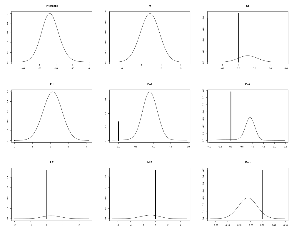
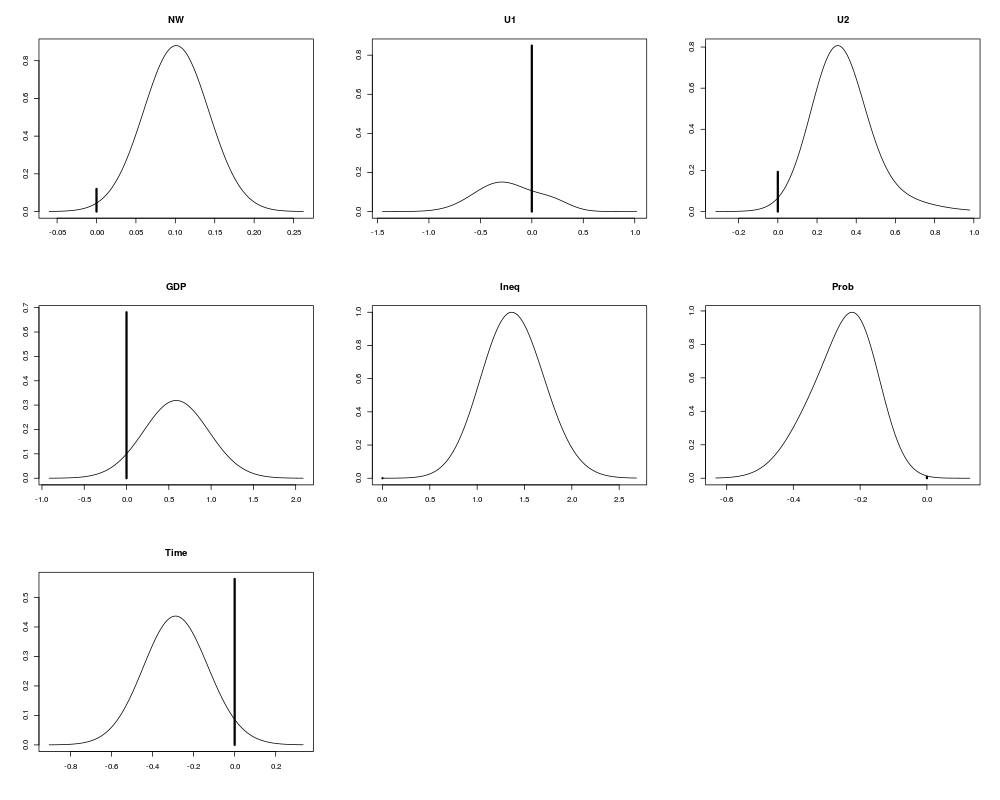
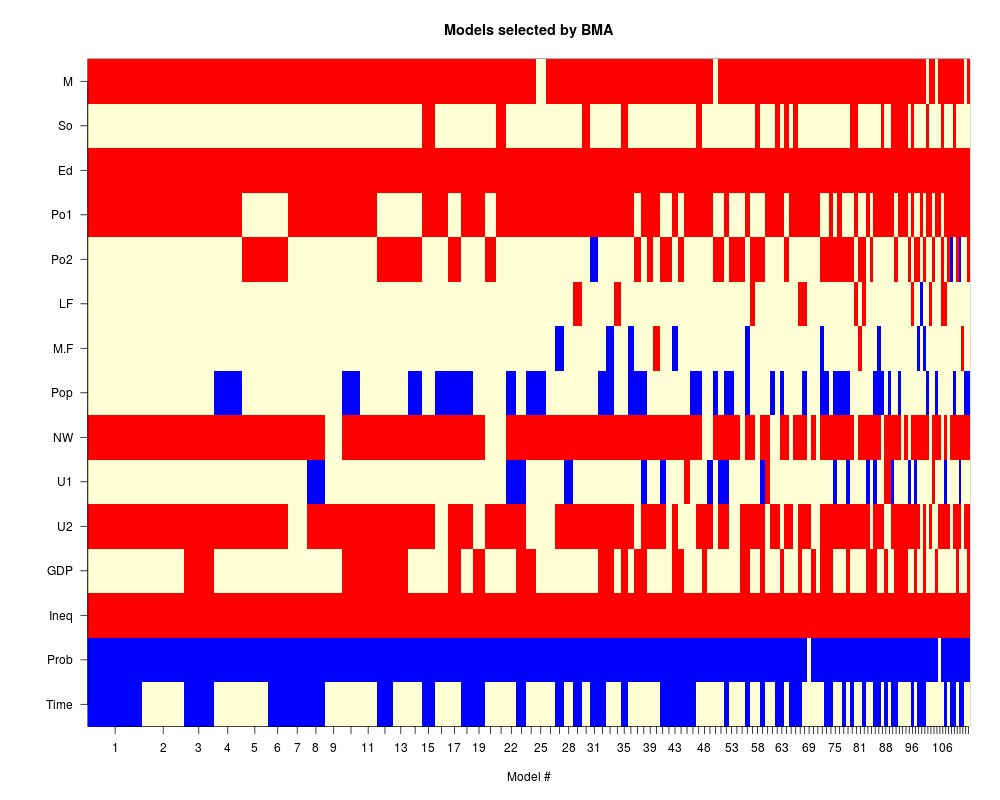
Examples

library(MASS)
data(UScrime)
x<- UScrime[,-16]
y<- log(UScrime[,16])
x[,-2]<- log(x[,-2])
lma<- bicreg(x, y, strict = FALSE, OR = 20) 
summary(lma)
plot(lma)

imageplot.bma(lma)

Results


R version 3.3.1 (2016-06-21) -- "Bug in Your Hair"
Copyright (C) 2016 The R Foundation for Statistical Computing
Platform: x86_64-pc-linux-gnu (64-bit)

R is free software and comes with ABSOLUTELY NO WARRANTY.
You are welcome to redistribute it under certain conditions.
Type 'license()' or 'licence()' for distribution details.

R is a collaborative project with many contributors.
Type 'contributors()' for more information and
'citation()' on how to cite R or R packages in publications.

Type 'demo()' for some demos, 'help()' for on-line help, or
'help.start()' for an HTML browser interface to help.
Type 'q()' to quit R.

> library(BMA)
Loading required package: survival
Loading required package: leaps
Loading required package: robustbase

Attaching package: 'robustbase'

The following object is masked from 'package:survival':

    heart

Loading required package: inline
Loading required package: rrcov
Scalable Robust Estimators with High Breakdown Point (version 1.3-11)

> png(filename="/home/ddbj/snapshot/RGM3/R_CC/result/BMA/bicreg.Rd_%03d_medium.png", width=480, height=480)
> ### Name: bicreg
> ### Title: Bayesian Model Averaging for linear regression models.
> ### Aliases: bicreg
> ### Keywords: regression models
> 
> ### ** Examples
> 
> library(MASS)
> data(UScrime)
> x<- UScrime[,-16]
> y<- log(UScrime[,16])
> x[,-2]<- log(x[,-2])
> lma<- bicreg(x, y, strict = FALSE, OR = 20) 
> summary(lma)

Call:
bicreg(x = x, y = y, strict = FALSE, OR = 20)


  115  models were selected
 Best  5  models (cumulative posterior probability =  0.2039 ): 

           p!=0    EV        SD       model 1    model 2    model 3  
Intercept  100.0  -23.45301  5.58897  -22.63715  -24.38362  -25.94554
M           97.3    1.38103  0.53531    1.47803    1.51437    1.60455
So          11.7    0.01398  0.05640      .          .          .    
Ed         100.0    2.12101  0.52527    2.22117    2.38935    1.99973
Po1         72.2    0.64849  0.46544    0.85244    0.91047    0.73577
Po2         32.0    0.24735  0.43829      .          .          .    
LF           6.0    0.01834  0.16242      .          .          .    
M.F          7.0   -0.06285  0.46566      .          .          .    
Pop         30.1   -0.01862  0.03626      .          .          .    
NW          88.0    0.08894  0.05089    0.10888    0.08456    0.11191
U1          15.1   -0.03282  0.14586      .          .          .    
U2          80.7    0.26761  0.19882    0.28874    0.32169    0.27422
GDP         31.9    0.18726  0.34986      .          .        0.54105
Ineq       100.0    1.38180  0.33460    1.23775    1.23088    1.41942
Prob        99.2   -0.24962  0.09999   -0.31040   -0.19062   -0.29989
Time        43.7   -0.12463  0.17627   -0.28659      .       -0.29682
                                                                     
nVar                                      8          7          9    
r2                                      0.842      0.826      0.851  
BIC                                   -55.91243  -55.36499  -54.69225
post prob                               0.062      0.047      0.034  
           model 4    model 5  
Intercept  -22.80644  -24.50477
M            1.26830    1.46061
So             .          .    
Ed           2.17788    2.39875
Po1          0.98597      .    
Po2            .        0.90689
LF             .          .    
M.F            .          .    
Pop         -0.05685      .    
NW           0.09745    0.08534
U1             .          .    
U2           0.28054    0.32977
GDP            .          .    
Ineq         1.32157    1.29370
Prob        -0.21636   -0.20614
Time           .          .    
                               
nVar           8          7    
r2           0.838      0.823  
BIC        -54.60434  -54.40788
post prob    0.032      0.029  
> plot(lma)
> 
> imageplot.bma(lma)
> 
> 
> 
> 
> 
> 
> dev.off()
null device 
          1 
>