Plots the posterior distributions of coefficients derived from Bayesian model averaging

Description

Displays plots of the posterior distributions of the coefficients generated by Bayesian model averaging over linear regression, generalized linear and survival analysis models.

Usage

## S3 method for class 'bicreg'
plot(x, e = 1e-04, mfrow = NULL, 
      include = 1:x$n.vars, include.intercept = TRUE, ...)

## S3 method for class 'bic.glm'
plot(x, e = 1e-04, mfrow = NULL, 
                       include = 1:length(x$namesx), ...)

## S3 method for class 'bic.surv'
plot(x, e = 1e-04, mfrow = NULL, 
                        include = 1:length(x$namesx), ...)

Arguments

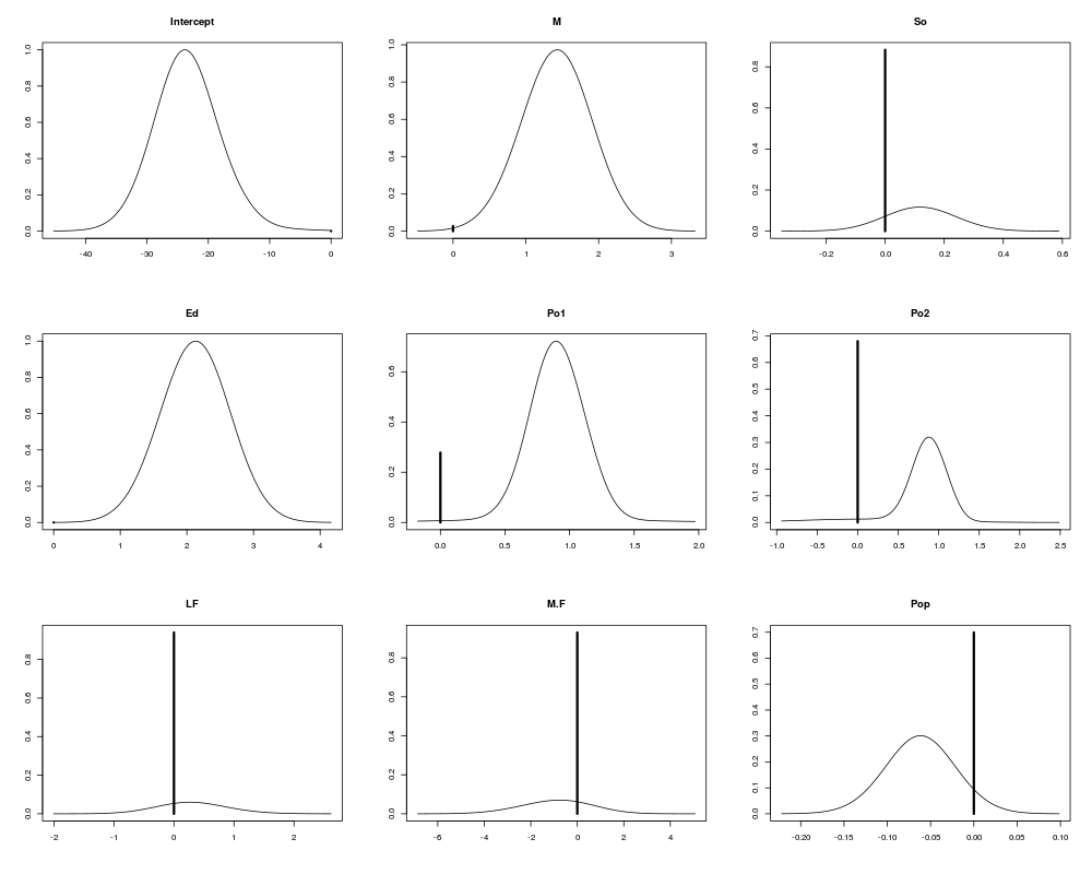
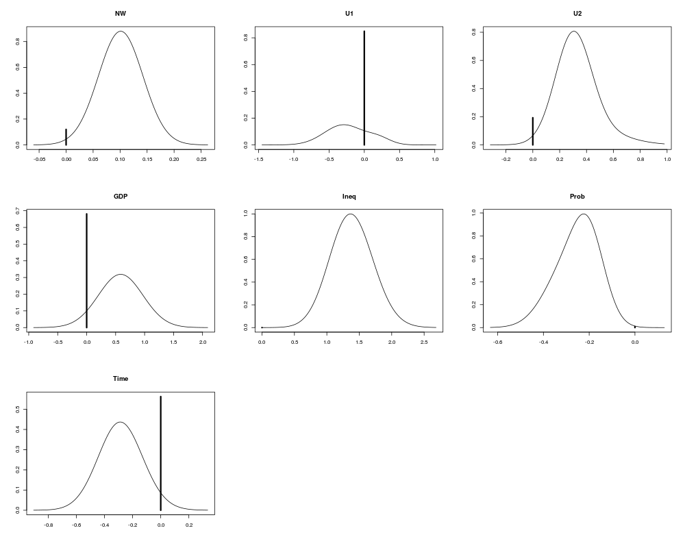
Details

Produces a plot of the posterior distribuion of the coefficients produced by model averaging. The posterior probability that the coefficient is zero is represented by a solid line at zero, with height equal to the probability. The nonzero part of the distribution is scaled so that the maximum height is equal to the probability that the coefficient is nonzero.

The parameter e specifies the range over which the distributions are to be graphed by specifying the tail probabilities that dictate the range to plot over.

Author(s)

Ian Painter ian.painter@AT@gmail.com

References

Hoeting, J.A., Raftery, A.E. and Madigan, D. (1996). A method for simultaneous variable selection and outlier identification in linear regression. Computational Statistics and Data Analysis, 22, 251-270.

Examples

library(MASS)
data(UScrime)
x<- UScrime[,-16]
y<- log(UScrime[,16])
x[,-2]<- log(x[,-2])
plot( bicreg(x, y)) 

Results

R version 3.3.1 (2016-06-21) -- "Bug in Your Hair"
Copyright (C) 2016 The R Foundation for Statistical Computing
Platform: x86_64-pc-linux-gnu (64-bit)

R is free software and comes with ABSOLUTELY NO WARRANTY.
You are welcome to redistribute it under certain conditions.
Type 'license()' or 'licence()' for distribution details.

R is a collaborative project with many contributors.
Type 'contributors()' for more information and
'citation()' on how to cite R or R packages in publications.

Type 'demo()' for some demos, 'help()' for on-line help, or
'help.start()' for an HTML browser interface to help.
Type 'q()' to quit R.

> library(BMA)
Loading required package: survival
Loading required package: leaps
Loading required package: robustbase

Attaching package: 'robustbase'

The following object is masked from 'package:survival':

    heart

Loading required package: inline
Loading required package: rrcov
Scalable Robust Estimators with High Breakdown Point (version 1.3-11)

> png(filename="/home/ddbj/snapshot/RGM3/R_CC/result/BMA/plot.bic.Rd_%03d_medium.png", width=480, height=480)
> ### Name: plot.bicreg
> ### Title: Plots the posterior distributions of coefficients derived from
> ###   Bayesian model averaging
> ### Aliases: plot.bicreg plot.bic.glm plot.bic.surv plot
> ### Keywords: regression models
> 
> ### ** Examples
> 
> library(MASS)
> data(UScrime)
> x<- UScrime[,-16]
> y<- log(UScrime[,16])
> x[,-2]<- log(x[,-2])
> plot( bicreg(x, y)) 
> 
> 
> 
> 
> 
> dev.off()
null device 
          1 
>