Transform confidence intervals from glm fits.

Description

Transform confidence intervals derived from glm fits back to original scale and give appropriate names.

Usage

## S3 method for class 'glht'
UnlogCI(x)

Arguments

Details

Applies exponential function on the estimates and confidence limits and creates useful names for the comparisons and parameters.

Value

An object of class "UnlogCI".

See Also

plotCI.UnlogCI for plotting the result

Examples

# # # CI for odds ratios
# # # for models on the logit-link

data(Feeding)

# Larval mortality:

Feeding$Lmort <- Feeding$Total - Feeding$Pupating

fit1<-glm(cbind(Pupating,Lmort)~Variety,data=Feeding, family=quasibinomial)
anova(fit1, test="F")

library(multcomp)

comp<-glht(fit1, mcp(Variety="Tukey"))

CIraw<-CIGLM(comp,method="Raw")

CIraw

UnlogCI(CIraw)

plotCI(UnlogCI(CIraw), lines=c(0.25,0.5,2,4),
 lineslwd=c(1,2,2,1), linescol=c("red","black","black","red"))


# # # # # # #

# # #  CI for ratios of means
# # # for models on the log-link

data(Diptera)

# Larval mortality:

fit2<-glm(Ges~Treatment, data=Diptera, family=quasipoisson)
anova(fit2, test="F")

library(multcomp)

comp<-glht(fit2, mcp(Treatment="Tukey"))

CIadj<-CIGLM(comp,method="Adj")

CIadj

UnlogCI(CIadj)

plotCI(UnlogCI(CIadj), lines=c(0.5,1,2), lineslwd=c(2,1,1))

Results

R version 3.3.1 (2016-06-21) -- "Bug in Your Hair"
Copyright (C) 2016 The R Foundation for Statistical Computing
Platform: x86_64-pc-linux-gnu (64-bit)

R is free software and comes with ABSOLUTELY NO WARRANTY.
You are welcome to redistribute it under certain conditions.
Type 'license()' or 'licence()' for distribution details.

R is a collaborative project with many contributors.
Type 'contributors()' for more information and
'citation()' on how to cite R or R packages in publications.

Type 'demo()' for some demos, 'help()' for on-line help, or
'help.start()' for an HTML browser interface to help.
Type 'q()' to quit R.

> library(BSagri)
Loading required package: gamlss
Loading required package: splines
Loading required package: gamlss.data
Loading required package: gamlss.dist
Loading required package: MASS
Loading required package: nlme
Loading required package: parallel
 **********   GAMLSS Version 4.4-0  ********** 
For more on GAMLSS look at http://www.gamlss.org/
Type gamlssNews() to see new features/changes/bug fixes.

Loading required package: multcomp
Loading required package: mvtnorm
Loading required package: survival

Attaching package: 'survival'

The following object is masked from 'package:gamlss.data':

    leukemia

Loading required package: TH.data

Attaching package: 'TH.data'

The following object is masked from 'package:MASS':

    geyser

Loading required package: MCPAN
> png(filename="/home/ddbj/snapshot/RGM3/R_CC/result/BSagri/UnlogCI.Rd_%03d_medium.png", width=480, height=480)
> ### Name: UnlogCI
> ### Title: Transform confidence intervals from glm fits.
> ### Aliases: UnlogCI UnlogCI.glht
> ### Keywords: htest
> 
> ### ** Examples
> 
> 
> # # # CI for odds ratios
> # # # for models on the logit-link
> 
> data(Feeding)
> 
> # Larval mortality:
> 
> Feeding$Lmort <- Feeding$Total - Feeding$Pupating
> 
> fit1<-glm(cbind(Pupating,Lmort)~Variety,data=Feeding, family=quasibinomial)
> anova(fit1, test="F")
Analysis of Deviance Table

Model: quasibinomial, link: logit

Response: cbind(Pupating, Lmort)

Terms added sequentially (first to last)


        Df Deviance Resid. Df Resid. Dev      F Pr(>F)
NULL                       31     59.623              
Variety  3   3.3623        28     56.260 0.6478 0.5909
> 
> library(multcomp)
> 
> comp<-glht(fit1, mcp(Variety="Tukey"))
> 
> CIraw<-CIGLM(comp,method="Raw")
> 
> CIraw

	 Simultaneous Confidence Intervals

Multiple Comparisons of Means: Tukey Contrasts


Fit: glm(formula = cbind(Pupating, Lmort) ~ Variety, family = quasibinomial, 
    data = Feeding)

Quantile = 1.96
95% confidence level
 

Linear Hypotheses:
                       Estimate lwr      upr     
S2 - S1 == 0           -0.18768 -1.10029  0.72493
NStandard - S1 == 0     0.06289 -0.85152  0.97729
Novum - S1 == 0         0.45291 -0.47882  1.38465
NStandard - S2 == 0     0.25057 -0.66316  1.16431
Novum - S2 == 0         0.64060 -0.29048  1.57168
Novum - NStandard == 0  0.39003 -0.54281  1.32287

> 
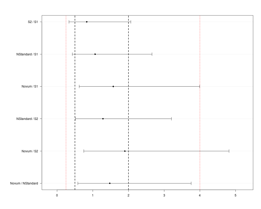
> UnlogCI(CIraw)
glm(formula = cbind(Pupating, Lmort) ~ Variety, family = quasibinomial, 
    data = Feeding)
Confidence intervals for odds ratios
with the odds defined as p(Pupating)/(1-p(Pupating)) 
                  Estimate   lwr   upr
S2 / S1              0.829 0.333 2.065
NStandard / S1       1.065 0.427 2.657
Novum / S1           1.573 0.620 3.993
NStandard / S2       1.285 0.515 3.204
Novum / S2           1.898 0.748 4.815
Novum / NStandard    1.477 0.581 3.754
Estimated quantile =  1.96 
> 
> plotCI(UnlogCI(CIraw), lines=c(0.25,0.5,2,4),
+  lineslwd=c(1,2,2,1), linescol=c("red","black","black","red"))
> 
> 
> # # # # # # #
> 
> # # #  CI for ratios of means
> # # # for models on the log-link
> 
> data(Diptera)
> 
> # Larval mortality:
> 
> fit2<-glm(Ges~Treatment, data=Diptera, family=quasipoisson)
> anova(fit2, test="F")
Analysis of Deviance Table

Model: quasipoisson, link: log

Response: Ges

Terms added sequentially (first to last)


          Df Deviance Resid. Df Resid. Dev      F  Pr(>F)  
NULL                         31     621.12                 
Treatment  3   145.62        28     475.50 2.6403 0.06892 .
---
Signif. codes:  0 '***' 0.001 '**' 0.01 '*' 0.05 '.' 0.1 ' ' 1
> 
> library(multcomp)
> 
> comp<-glht(fit2, mcp(Treatment="Tukey"))
> 
> CIadj<-CIGLM(comp,method="Adj")
> 
> CIadj

	 Simultaneous Confidence Intervals

Multiple Comparisons of Means: Tukey Contrasts


Fit: glm(formula = Ges ~ Treatment, family = quasipoisson, data = Diptera)

Quantile = 2.5664
95% family-wise confidence level
 

Linear Hypotheses:
                    Estimate lwr      upr     
S2 - S1 == 0        -0.40637 -1.14578  0.33305
SNovum - S1 == 0    -0.50303 -1.26464  0.25857
Novum - S1 == 0      0.16900 -0.46596  0.80395
SNovum - S2 == 0    -0.09667 -0.92710  0.73377
Novum - S2 == 0      0.57536 -0.14070  1.29143
Novum - SNovum == 0  0.67203 -0.06693  1.41099

> 
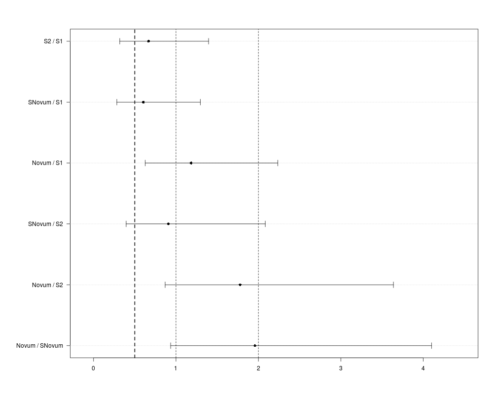
> UnlogCI(CIadj)
glm(formula = Ges ~ Treatment, family = quasipoisson, data = Diptera)
Confidence intervals for the ratios of abundance 
               Estimate   lwr   upr
S2 / S1           0.666 0.318 1.395
SNovum / S1       0.605 0.282 1.295
Novum / S1        1.184 0.628 2.234
SNovum / S2       0.908 0.396 2.083
Novum / S2        1.778 0.869 3.638
Novum / SNovum    1.958 0.935 4.100
Estimated quantile =  2.5664 
> 
> plotCI(UnlogCI(CIadj), lines=c(0.5,1,2), lineslwd=c(2,1,1))
> 
> 
> 
> 
> 
> 
> 
> dev.off()
null device 
          1 
>