R Graphical Manual

Browse All

Last data update: 2014.03.03

R: A default Bayesian hypothesis test for partial correlation...

jzs_partcorSD

R Documentation

A default Bayesian hypothesis test for partial correlation using the Savage-Dickey method.

Description

This function can be used to perform a default Bayesian hypothesis test for partial correlation, using the Savage-Dickey method (Dickey & Lientz, 1970). The test uses a Jeffreys-Zellner-Siow prior set-up (Liang et al., 2008).

Usage

jzs_partcorSD(V1, V2, control, 
              SDmethod = c("fit.st", "dnorm", "splinefun", "logspline"),
              alternative = c("two.sided", "less", "greater"),
              n.iter=10000,n.burnin=500,standardize=TRUE)

Arguments

`V1`	a numeric vector.
`V2`	a numeric vector of the same length as V1.
`control`	a numeric vector of the same length as V1 and V2. This variable is partialled out of the correlation between V1 and V2.
`SDmethod`	specify the precise method with which the density of the posterior distribution will be estimated in order to compute the Savage-Dickey ratio.
`alternative`	specify the alternative hypothesis for the correlation coefficient: `two.sided`, `greater` than zero, or `less` than zero.
`n.iter`	number of total iterations per chain (see the package `R2jags`). Defaults to 10000.
`n.burnin`	length of burn in, i.e. number of iterations to discard at the beginning(see the package `R2jags`). Defaults to 500.
`standardize`	logical. Should the variables be standardized? Defaults to TRUE.

Value

`PartCoef`	Mean of the posterior samples of the unstandardized partial correlation (the regression coefficient beta in the equation V2 = intercept + alphacontrol + betaV1).
`BayesFactor`	The Bayes factor for the correlation coefficient. A value greater than one indicates evidence in favor of correlation, a value smaller than one indicates evidence against correlation.
`PosteriorProbability`	The posterior probability for the existence of a correlation between V1 and V2.
`beta`	The posterior samples for the regression coefficient beta. This is the unstandardized partial correlation.
`jagssamples`	The JAGS output for the MCMC estimation of the path. This object can be used to construct a traceplot.

Warning

In some cases the SDmethod fit.st will fail to converge. If so, another optimization method is used, using different starting values. If the other optimization method does not converge either or gives you a negative Bayes factor (which is meaningless), you could try one of the other SDmethod options or see jzs_partcor.

Author(s)

Michele B. Nuijten <m.b.nuijten@uvt.nl>, Ruud Wetzels, Dora Matzke, Conor V. Dolan, and Eric-Jan Wagenmakers.

References

Dickey, J. M., & Lientz, B. P. (1970). The weighted likelihood ratio, sharp hypotheses about chances, the order of a Markov chain. The Annals of Mathematical Statistics, 214-226.

Liang, F., Paulo, R., Molina, G., Clyde, M. A., & Berger, J. O. (2008). Mixtures of g priors for Bayesian variable selection. Journal of the American Statistical Association, 103(481), 410-423.

Nuijten, M. B., Wetzels, R., Matzke, D., Dolan, C. V., & Wagenmakers, E.-J. (2014). A default Bayesian hypothesis test for mediation. Behavior Research Methods. doi: 10.3758/s13428-014-0470-2

Wetzels, R., & Wagenmakers, E.-J. (2012). A Default Bayesian Hypothesis Test for Correlations and Partial Correlations. Psychonomic Bulletin & Review, 19, 1057-1064.

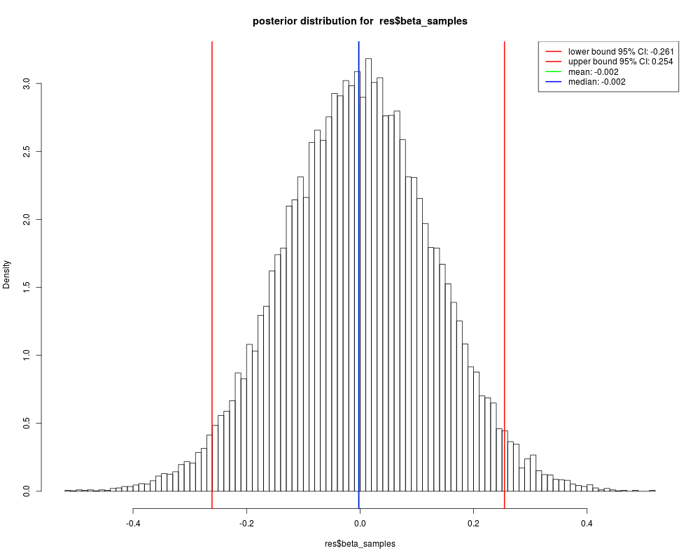
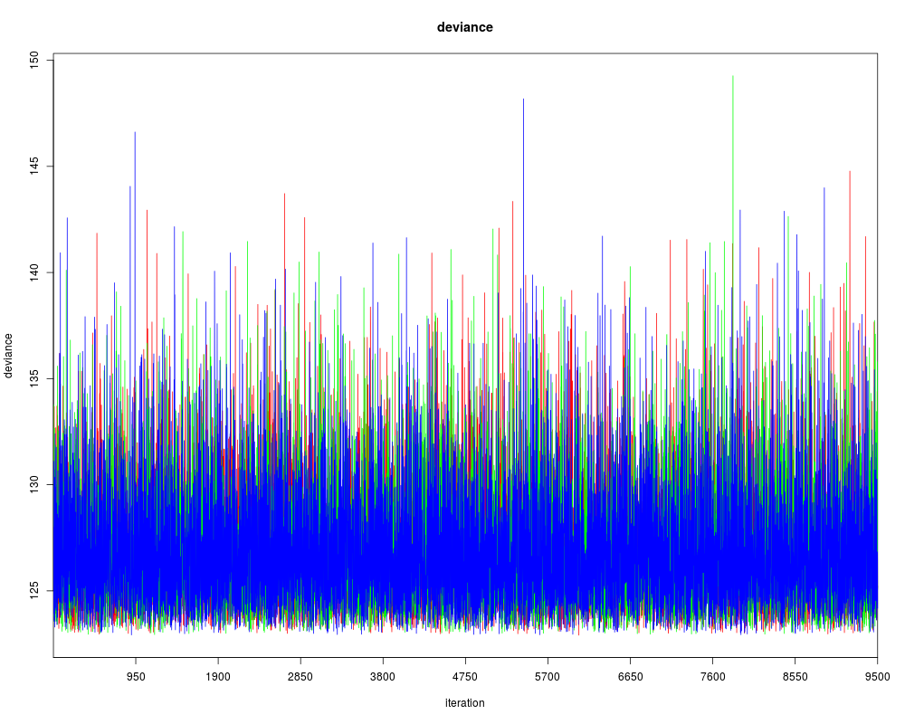
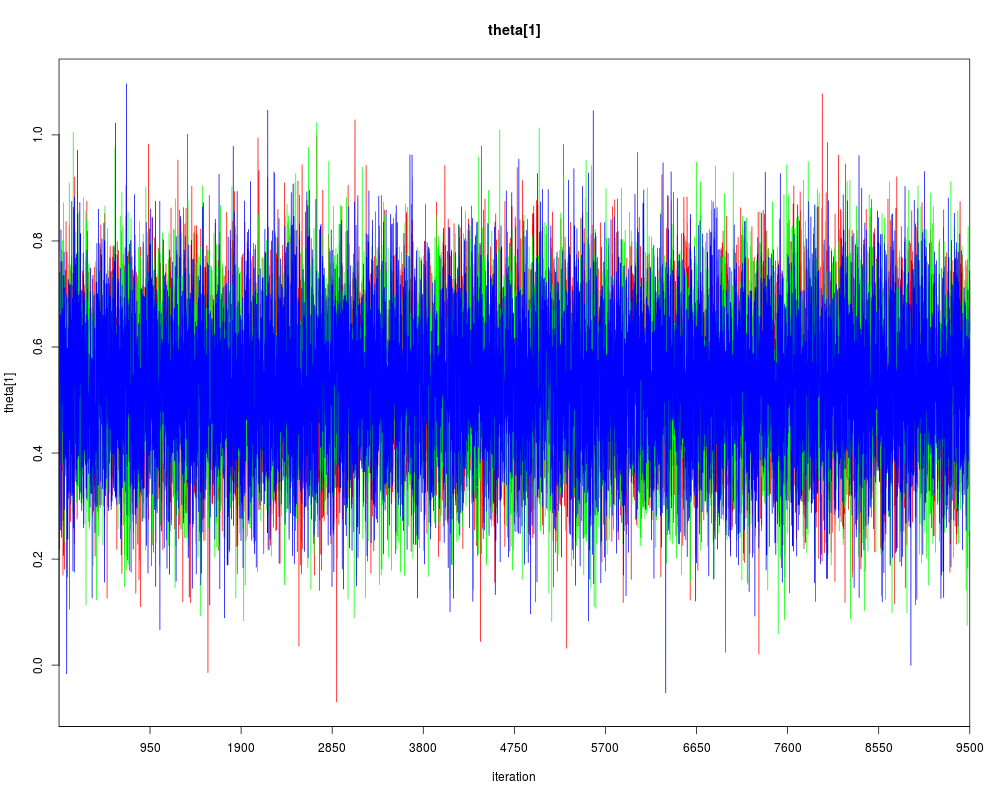
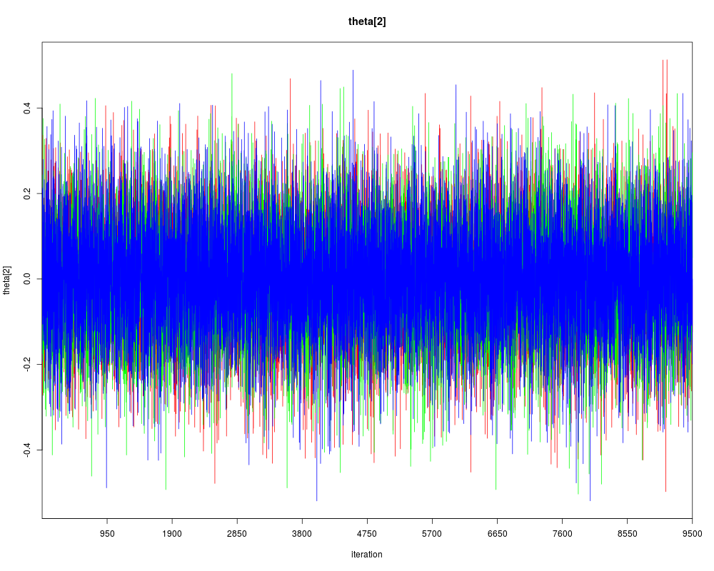
Examples

# simulate partially correlated data
X <- rnorm(50,0,1)
C <- .5*X + rnorm(50,0,1)
Y <- .3*X + .6*C + rnorm(50,0,1)

# run jzs_partcor
(res <- jzs_partcorSD(X,Y,C))

# plot posterior samples
plot(res$beta_samples)

# plot traceplot
plot(res$jagssamples)
# where the first chain (theta[1]) is for tau' and the second chain (theta[2]) for beta

Results


R version 3.3.1 (2016-06-21) -- "Bug in Your Hair"
Copyright (C) 2016 The R Foundation for Statistical Computing
Platform: x86_64-pc-linux-gnu (64-bit)

R is free software and comes with ABSOLUTELY NO WARRANTY.
You are welcome to redistribute it under certain conditions.
Type 'license()' or 'licence()' for distribution details.

R is a collaborative project with many contributors.
Type 'contributors()' for more information and
'citation()' on how to cite R or R packages in publications.

Type 'demo()' for some demos, 'help()' for on-line help, or
'help.start()' for an HTML browser interface to help.
Type 'q()' to quit R.

> library(BayesMed)
Loading required package: R2jags
Loading required package: rjags
Loading required package: coda
Linked to JAGS 4.1.0
Loaded modules: basemod,bugs

Attaching package: 'R2jags'

The following object is masked from 'package:coda':

    traceplot

Loading required package: QRM
Loading required package: gsl
Loading required package: Matrix
Loading required package: mvtnorm
Loading required package: numDeriv
Loading required package: timeSeries
Loading required package: timeDate

Attaching package: 'QRM'

The following object is masked from 'package:base':

    lbeta

Loading required package: polspline
Loading required package: MCMCpack
Loading required package: MASS
##
## Markov Chain Monte Carlo Package (MCMCpack)
## Copyright (C) 2003-2016 Andrew D. Martin, Kevin M. Quinn, and Jong Hee Park
##
## Support provided by the U.S. National Science Foundation
## (Grants SES-0350646 and SES-0350613)
##
> png(filename="/home/ddbj/snapshot/RGM3/R_CC/result/BayesMed/jzs_partcorSD.Rd_%03d_medium.png", width=480, height=480)
> ### Name: jzs_partcorSD
> ### Title: A default Bayesian hypothesis test for partial correlation using
> ###   the Savage-Dickey method.
> ### Aliases: jzs_partcorSD
> 
> ### ** Examples
> 
> # simulate partially correlated data
> X <- rnorm(50,0,1)
> C <- .5*X + rnorm(50,0,1)
> Y <- .3*X + .6*C + rnorm(50,0,1)
> 
> # run jzs_partcor
> (res <- jzs_partcorSD(X,Y,C))
module glm loaded
Compiling model graph
   Resolving undeclared variables
   Allocating nodes
Graph information:
   Observed stochastic nodes: 50
   Unobserved stochastic nodes: 4
   Total graph size: 339

Initializing model

$PartCoef
[1] 0.3188769

$BayesFactor
[1] 2.551363

$PosteriorProbability
[1] 0.7184179

> 
> # plot posterior samples
> plot(res$beta_samples)
> 
> # plot traceplot
> plot(res$jagssamples)
> # where the first chain (theta[1]) is for tau' and the second chain (theta[2]) for beta
> 
> 
> 
> 
> 
> dev.off()
null device 
          1 
>