(Slightly extended) Bland-Altman plots BlandAltmanLeh

Description

Bland-Altman Plots for assessing agreement between two methods of clinical measurement and returning associated statistics. Plots are optionally extended by confidence intervals as described in "J. Martin Bland, Douglas G. Altman (1986): Statistical Methods For Assessing Agreement Between Two Methods Of Clinical Measurement" but not included in the graphics of that publication. Either base graphics or ggplot2 can be used.

Details

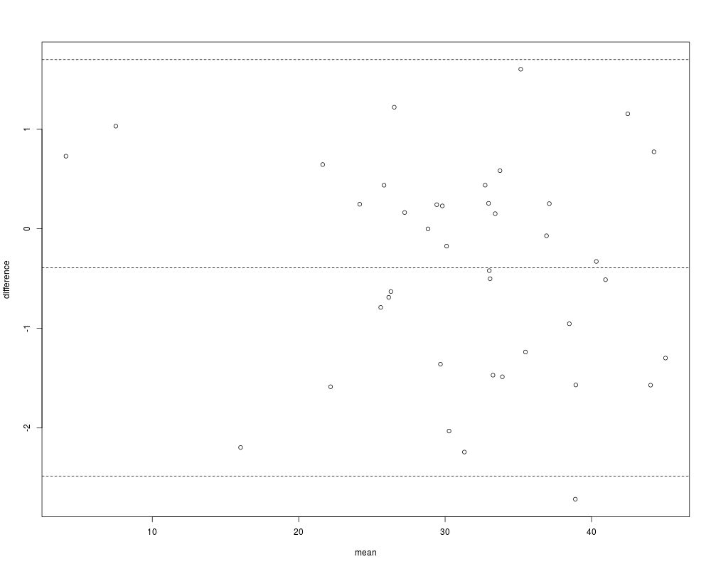
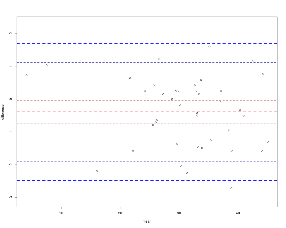
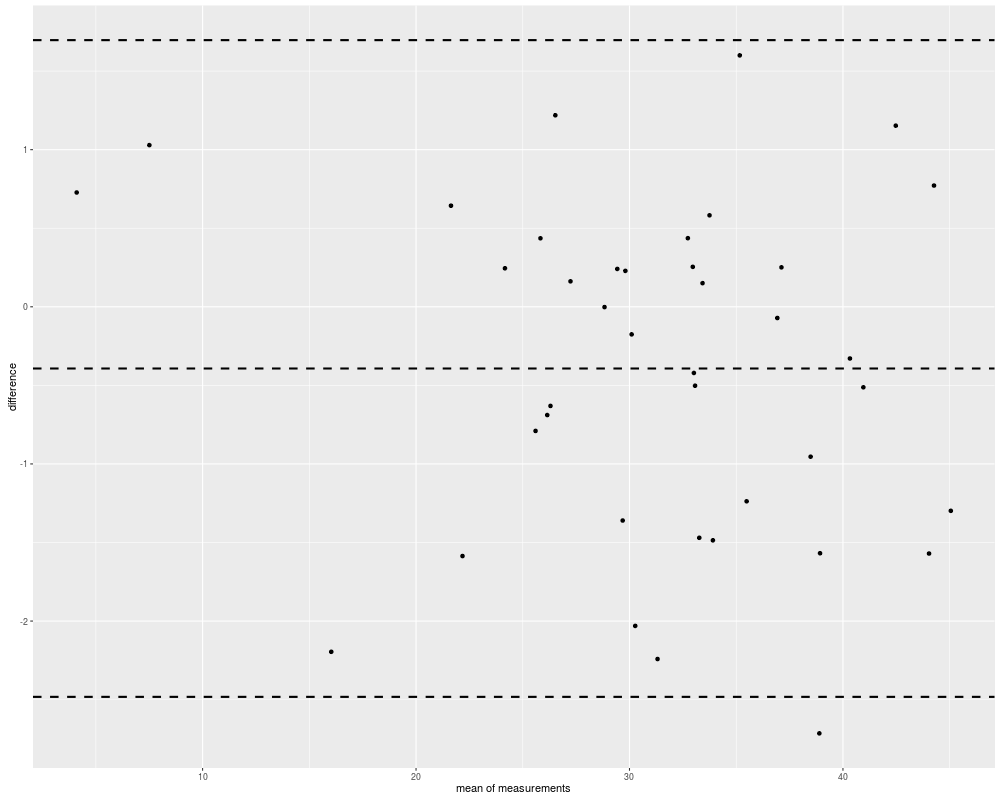
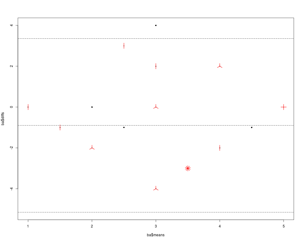
Bland Altman plots are a diagnostic tool for assessing the agreement between two methods of measurement or assessing retest reliability from two measurements. This package offers plots in base and ggplot2 graphics as well as detailed descriptive statistics, thus supporting the construction of individual plots based on Bland Altman plots. Bland and Altman describe a way for constructing confidence intervals. This package computes these confidence intervals and includes them into the plots. It also invents the Sunflower-Bland-Altman plot for data with ties.

Author(s)

Bernhard Lehnert

Maintainer: Bernhard K. Lehnert <bernhard.lehnert@uni-greifswald.de>

References

Bland JM, Altman DG, Statistical Methods For Assessing Agreement Between Two Methods Of Clinical Measurement, Lancet, 1986; 307-310.

Altman DG, Bland JM, Measurement in medicine: the analysis of method comparison studies, The Statistician 1983; 32, 307-317.

Vaz S et al., The Case for Using the Repeatability Coeffcient When Calculating Test-Retest Reliability, PLOS ONE, Sept. 2013, Vol 8, Issue 9.

See Also

bland.altman.plot,bland.altman.stats

Examples

# simple basic Bland Altman plot
a <- rnorm(40,30,10)
b <- 1.01*a + rnorm(40)
bland.altman.plot(a,b, xlab="mean", ylab="difference")

# to get all the data for further analysis
bland.altman.plot(a,b, xlab="mean", ylab="difference", silent=FALSE)

# to include confidence intervals into the plot
bland.altman.plot(a,b, xlab="mean", ylab="difference", conf.int=.95)

# to plot in ggplot2
bland.altman.plot(a,b, graph.sys="ggplot2")

# to mark ties in a Sunflower-Bland-Altman plot
a <- sample(1:5, 40, replace=TRUE)
b <- rep(c(1,2,3,3,5,5,5,5),5)
bland.altman.plot(a, b, sunflower=TRUE)
 

Results

R version 3.3.1 (2016-06-21) -- "Bug in Your Hair"
Copyright (C) 2016 The R Foundation for Statistical Computing
Platform: x86_64-pc-linux-gnu (64-bit)

R is free software and comes with ABSOLUTELY NO WARRANTY.
You are welcome to redistribute it under certain conditions.
Type 'license()' or 'licence()' for distribution details.

R is a collaborative project with many contributors.
Type 'contributors()' for more information and
'citation()' on how to cite R or R packages in publications.

Type 'demo()' for some demos, 'help()' for on-line help, or
'help.start()' for an HTML browser interface to help.
Type 'q()' to quit R.

> library(BlandAltmanLeh)
> png(filename="/home/ddbj/snapshot/RGM3/R_CC/result/BlandAltmanLeh/BlandAltmanLeh-package.Rd_%03d_medium.png", width=480, height=480)
> ### Name: BlandAltmanLeh-package
> ### Title: (Slightly extended) Bland-Altman plots BlandAltmanLeh
> ### Aliases: BlandAltmanLeh-package BlandAltmanLeh
> ### Keywords: measurement precision, test-retest reliability
> 
> ### ** Examples
> 
> # simple basic Bland Altman plot
> a <- rnorm(40,30,10)
> b <- 1.01*a + rnorm(40)
> bland.altman.plot(a,b, xlab="mean", ylab="difference")
NULL
> 
> # to get all the data for further analysis
> bland.altman.plot(a,b, xlab="mean", ylab="difference", silent=FALSE)
$means
 [1] 45.921259 45.314504 23.931613 37.637122 19.089934 30.250768 28.187797
 [8] 37.922317 26.176296 15.939471 32.009322 26.582369 13.310724 15.103460
[15] 33.669045 36.590791 31.084450 36.941137 38.996712 41.229372 21.744200
[22] 32.631554 31.322151 40.616027 31.047996 46.254833 21.643849 37.981818
[29] 23.664460 34.673067 30.644141 21.854745 28.017781 45.689398 47.911303
[36] 26.445259 17.894171 25.424877 39.194830  3.248392

$diffs
 [1] -0.82627267 -2.19265843 -1.00250467 -1.22793677 -0.16367574 -0.82884285
 [7] -0.59721152 -0.35915349 -0.77556529  2.24255612  1.09322934 -0.51103489
[13] -0.52194274 -1.48134323  0.12579402  0.77498039 -1.58275657 -0.63040641
[19]  0.20439908 -1.60779801  2.09226805  0.01986367  0.70874247 -0.27262528
[25] -1.12556682 -1.39279705  0.29365889 -0.12249887  0.43522737 -0.03814481
[31]  1.27887843 -1.67963327 -0.52624544  0.62029513 -1.12946647 -1.73602221
[37] -0.14951021  1.41346483  1.30760400 -0.48480071

$groups
      group1    group2
1  45.508123 46.334396
2  44.218175 46.410834
3  23.430361 24.432866
4  37.023154 38.251091
5  19.008096 19.171772
6  29.836346 30.665189
7  27.889191 28.486403
8  37.742740 38.101894
9  25.788513 26.564079
10 17.060749 14.818193
11 32.555937 31.462708
12 26.326852 26.837887
13 13.049752 13.571695
14 14.362789 15.844132
15 33.731942 33.606148
16 36.978281 36.203301
17 30.293072 31.875828
18 36.625934 37.256341
19 39.098911 38.894512
20 40.425473 42.033271
21 22.790334 20.698066
22 32.641486 32.621622
23 31.676522 30.967780
24 40.479715 40.752340
25 30.485213 31.610780
26 45.558434 46.951231
27 21.790679 21.497020
28 37.920568 38.043067
29 23.882074 23.446847
30 34.653995 34.692140
31 31.283580 30.004701
32 21.014928 22.694562
33 27.754659 28.280904
34 45.999546 45.379250
35 47.346570 48.476037
36 25.577248 27.313271
37 17.819416 17.968926
38 26.131609 24.718144
39 39.848632 38.541028
40  3.005992  3.490793

$based.on
[1] 40

$lower.limit
[1] -2.341869

$mean.diffs
[1] -0.2588863

$upper.limit
[1] 1.824096

$lines
lower.limit  mean.diffs upper.limit 
 -2.3418690  -0.2588863   1.8240964 

$CI.lines
lower.limit.ci.lower lower.limit.ci.upper   mean.diff.ci.lower 
          -2.3418690           -2.3418690           -0.2588863 
  mean.diff.ci.upper upper.limit.ci.lower upper.limit.ci.upper 
          -0.2588863            1.8240964            1.8240964 

$two
[1] 1.96

$critical.diff
[1] 2.082983

> 
> # to include confidence intervals into the plot
> bland.altman.plot(a,b, xlab="mean", ylab="difference", conf.int=.95)
NULL
> 
> # to plot in ggplot2
> bland.altman.plot(a,b, graph.sys="ggplot2")
Loading required namespace: ggplot2
> 
> # to mark ties in a Sunflower-Bland-Altman plot
> a <- sample(1:5, 40, replace=TRUE)
> b <- rep(c(1,2,3,3,5,5,5,5),5)
> bland.altman.plot(a, b, sunflower=TRUE)
NULL
>  
> 
> 
> 
> 
> 
> dev.off()
null device 
          1 
>