R Graphical Manual

Browse All

Last data update: 2014.03.03

R: Bayesian inference for simple linear regression

bayes.lin.reg

R Documentation

Bayesian inference for simple linear regression

Description

This function is used to find the posterior distribution of the simple linear regression slope variable beta when we have a random sample of ordered pairs (x_{i}, y_{i}) from the simple linear regression model:

y_i = alpha_xbar + beta*x_i+epsilon_i

where the observation errors are, epsilon_i, independent normal(0,sigma^2) with known variance.

Usage

bayes.lin.reg(y, x, slope.prior = "flat", intcpt.prior = "flat", mb0 = 0,
  sb0 = 0, ma0 = 0, sa0 = 0, sigma = NULL, alpha = 0.05,
  plot.data = FALSE, pred.x = NULL)

Arguments

`y`	the vector of responses.
`x`	the value of the explantory variable associated with each response.
`slope.prior`	use a “flat” prior or a “normal” prior. for beta
`intcpt.prior`	use a “flat” prior or a “normal” prior. for alpha_xbar
`mb0`	the prior mean of the simple linear regression slope variable beta. This argument is ignored for a flat prior.
`sb0`	the prior std. deviation of the simple linear regression slope variable beta - must be greater than zero. This argument is ignored for a flat prior.
`ma0`	the prior mean of the simple linear regression intercept variable alpha_xbar. This argument is ignored for a flat prior.
`sa0`	the prior std. deviation of the simple linear regression variable alpha_xbar - must be greater than zero. This argument is ignored for a flat prior.
`sigma`	the value of the std. deviation of the residuals. By default, this is assumed to be unknown and the sample value is used instead. This affects the prediction intervals.
`alpha`	controls the width of the credible interval.
`plot.data`	if true the data are plotted, and the posterior regression line superimposed on the data.
`pred.x`	a vector of x values for which the predicted y values are obtained and the std. errors of prediction

Value

A list will be returned with the following components:

`post.coef`	the posterior mean of the intecept and the slope
`post.coef`	the posterior standard deviation of the intercept the slope
`pred.x`	the vector of values for which predictions have been requested. If pred.x is NULL then this is not returned
`pred.y`	the vector predicted values corresponding to pred.x. If pred.x is NULL then this is not returned
`pred.se`	The standard errors of the predicted values in pred.y. If pred.x is NULL then this is not returned

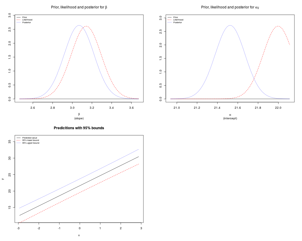
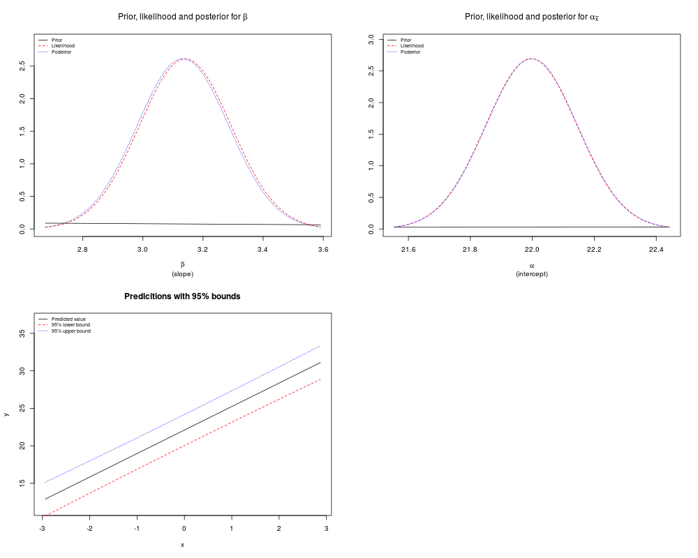
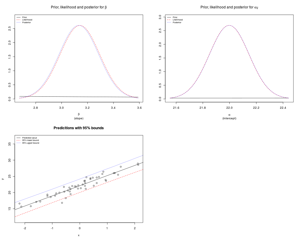
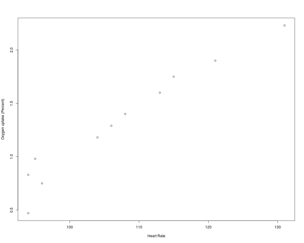
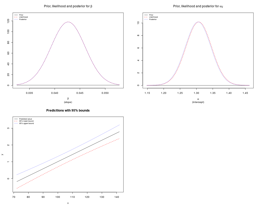
Examples


## generate some data from a known model, where the true value of the
## intercept alpha is 2, the true value of the slope beta is 3, and the
## errors come from a normal(0,1) distribution
x = rnorm(50)
y = 22+3*x+rnorm(50)

## use the function with a flat prior for the slope beta and a
## flat prior for the intercept, alpha_xbar.

bayes.lin.reg(y,x)

## use the function with a normal(0,3) prior for the slope beta and a
## normal(30,10) prior for the intercept, alpha_xbar.

bayes.lin.reg(y,x,"n","n",0,3,30,10)

## use the same data but plot it and the credible interval

bayes.lin.reg(y,x,"n","n",0,3,30,10, plot.data = TRUE)

## The heart rate vs. O2 uptake example 14.1
O2 = c(0.47,0.75,0.83,0.98,1.18,1.29,1.40,1.60,1.75,1.90,2.23)
HR = c(94,96,94,95,104,106,108,113,115,121,131)
plot(HR,O2,xlab="Heart Rate",ylab="Oxygen uptake (Percent)")

bayes.lin.reg(O2,HR,"n","f",0,1,sigma=0.13)

## Repeat the example but obtain predictions for HR = 100 and 110

bayes.lin.reg(O2,HR,"n","f",0,1,sigma=0.13,pred.x=c(100,110))

Results


R version 3.3.1 (2016-06-21) -- "Bug in Your Hair"
Copyright (C) 2016 The R Foundation for Statistical Computing
Platform: x86_64-pc-linux-gnu (64-bit)

R is free software and comes with ABSOLUTELY NO WARRANTY.
You are welcome to redistribute it under certain conditions.
Type 'license()' or 'licence()' for distribution details.

R is a collaborative project with many contributors.
Type 'contributors()' for more information and
'citation()' on how to cite R or R packages in publications.

Type 'demo()' for some demos, 'help()' for on-line help, or
'help.start()' for an HTML browser interface to help.
Type 'q()' to quit R.

> library(Bolstad)

Attaching package: 'Bolstad'

The following objects are masked from 'package:stats':

    IQR, sd, var

> png(filename="/home/ddbj/snapshot/RGM3/R_CC/result/Bolstad/bayes.lin.reg.Rd_%03d_medium.png", width=480, height=480)
> ### Name: bayes.lin.reg
> ### Title: Bayesian inference for simple linear regression
> ### Aliases: bayes.lin.reg
> ### Keywords: misc
> 
> ### ** Examples
> 
> 
> ## generate some data from a known model, where the true value of the
> ## intercept alpha is 2, the true value of the slope beta is 3, and the
> ## errors come from a normal(0,1) distribution
> x = rnorm(50)
> y = 22+3*x+rnorm(50)
> 
> ## use the function with a flat prior for the slope beta and a
> ## flat prior for the intercept, alpha_xbar.
> 
> bayes.lin.reg(y,x)
Standard deviation of residuals:  0.985 
            Posterior Mean Posterior Std. Deviation
            -------------- ------------------------
Intercept:  21.12          0.13794                 
Slope:      3.034          0.12511                 
> 
> ## use the function with a normal(0,3) prior for the slope beta and a
> ## normal(30,10) prior for the intercept, alpha_xbar.
> 
> bayes.lin.reg(y,x,"n","n",0,3,30,10)
Standard deviation of residuals:  0.985 
            Posterior Mean Posterior Std. Deviation
            -------------- ------------------------
Intercept:  21.54          0.13926                 
Slope:      3.076          0.12599                 
> 
> ## use the same data but plot it and the credible interval
> 
> bayes.lin.reg(y,x,"n","n",0,3,30,10, plot.data = TRUE)
Standard deviation of residuals:  0.985 
            Posterior Mean Posterior Std. Deviation
            -------------- ------------------------
Intercept:  21.54          0.13926                 
Slope:      3.076          0.12599                 
> 
> ## The heart rate vs. O2 uptake example 14.1
> O2 = c(0.47,0.75,0.83,0.98,1.18,1.29,1.40,1.60,1.75,1.90,2.23)
> HR = c(94,96,94,95,104,106,108,113,115,121,131)
> plot(HR,O2,xlab="Heart Rate",ylab="Oxygen uptake (Percent)")
> 
> bayes.lin.reg(O2,HR,"n","f",0,1,sigma=0.13)
Known standard deviation:  0.13 
            Posterior Mean Posterior Std. Deviation
            -------------- ------------------------
Intercept:  1.305          0.039253                
Slope:      0.04265        0.0033798               
> 
> ## Repeat the example but obtain predictions for HR = 100 and 110
> 
> bayes.lin.reg(O2,HR,"n","f",0,1,sigma=0.13,pred.x=c(100,110))
Known standard deviation:  0.13 
            Posterior Mean Posterior Std. Deviation
            -------------- ------------------------
Intercept:  1.305          0.039253                
Slope:      0.04265        0.0033798               
x       Predicted y  SE         
------  -----------  -----------
100       1.007        0.13784    
110       1.433        0.13617    
> 
> 
> 
> 
> 
> 
> dev.off()
null device 
          1 
>