an optional (non-empty) numeric vector of data values.
alternative
a character string specifying the alternative hypothesis, must be one of
"two.sided" (default), "greater" or "less". You can specify just the initial
letter.
mu
a number indicating the true value of the mean (or difference in means if you are performing a two sample test).
paired
a logical indicating whether you want a paired t-test.
var.equal
a logical variable indicating whether to treat the two variances as being equal.
If TRUE (default) then the pooled variance is used to estimate the variance otherwise the
Welch (or Satterthwaite) approximation to the degrees of freedom is used. The unequal variance case is
implented using Gibbs sampling.
conf.level
confidence level of interval.
prior
a character string indicating which prior should be used for the means, must be one of
"jeffreys" (default) for independent Jeffreys' priors on the unknown mean(s) and variance(s),
or "joint.conj" for a joint conjugate prior.
m
if the joint conjugate prior is used then the user must specify a prior mean in the one-sample
or paired case, or two prior means in the two-sample case. Note that if the hypothesis is that there is no difference
between the means in the two-sample case, then the values of the prior means should usually be equal, and if so,
then their actual values are irrelvant.This parameter is not used if the user chooses a Jeffreys' prior.
n0
if the joint conjugate prior is used then the user must specify the prior precision
or precisions in the two sample case that represent our level of uncertainty
about the true mean(s). This parameter is not used if the user chooses a Jeffreys' prior.
sig.med
if the joint conjugate prior is used then the user must specify the prior median
for the unknown standard deviation. This parameter is not used if the user chooses a Jeffreys' prior.
kappa
if the joint conjugate prior is used then the user must specify the degrees of freedom
for the inverse chi-squared distribution used for the unknown standard deviation. Usually the default
of 1 will be sufficient. This parameter is not used if the user chooses a Jeffreys' prior.
sigmaPrior
If a two-sample t-test with unequal variances is desired then the user must choose between
using an chi-squared prior ("chisq") or a gamma prior ("gamma") for the unknown population standard deviations.
This parameter is only used if var.equal is set to FALSE.
nIter
Gibbs sampling is used when a two-sample t-test with unequal variances is desired.
This parameter controls the sample size from the posterior distribution.
nBurn
Gibbs sampling is used when a two-sample t-test with unequal variances is desired.
This parameter controls the number of iterations used to burn in the chains before the procedure
starts sampling in order to reduce correlation with the starting values.
formula
a formula of the form lhs ~ rhs where lhs is a numeric variable giving the data values and rhs a factor with two
levels giving the corresponding groups.
data
an optional matrix or data frame (or similar: see model.frame) containing
the variables in the formula formula. By default the variables are taken from environment(formula).
subset
currently ingored.
na.action
currently ignored.
Value
A list with class "htest" containing the following components:
statistic
the value of the t-statistic.
parameter
the degrees of freedom for the t-statistic.
p.value
the p-value for the test.
"
conf.int
a confidence interval for the mean appropriate to the specified alternative hypothesis.
estimate
the estimated mean or difference in means depending on whether it was a one-sample test or a two-sample test.
null.value
the specified hypothesized value of the mean or mean difference depending on whether it was a one-sample test or a two-sample test.
alternative
a character string describing the alternative hypothesis.
method
a character string indicating what type of t-test was performed.
data.name
a character string giving the name(s) of the data.
result
an object of class Bolstad
Methods (by class)
default: Bayesian t-test
formula: Bayesian t-test
Author(s)
R Core with Bayesian internals added by James Curran
Examples
bayes.t.test(1:10, y = c(7:20)) # P = .3.691e-01
## Same example but with using the joint conjugate prior
## We set the prior means equal (and it doesn't matter what the value is)
## the prior precision is 0.01, which is a prior standard deviation of 10
## we're saying the true difference of the means is between [-25.7, 25.7]
## with probability equal to 0.99. The median value for the prior on sigma is 2
## and we're using a scaled inverse chi-squared prior with 1 degree of freedom
bayes.t.test(1:10, y = c(7:20), var.equal = TRUE, prior = "joint.conj",
m = c(0,0), n0 = rep(0.01, 2), sig.med = 2)
##' Same example but with a large outlier. Note the assumption of equal variances isn't sensible
bayes.t.test(1:10, y = c(7:20, 200)) # P = .1979 -- NOT significant anymore
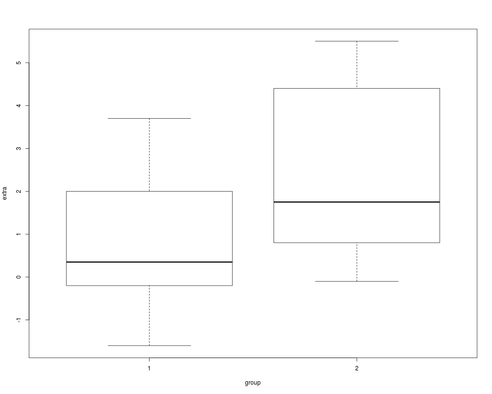
## Classical example: Student's sleep data
plot(extra ~ group, data = sleep)
## Traditional interface
with(sleep, bayes.t.test(extra[group == 1], extra[group == 2]))
## Formula interface
bayes.t.test(extra ~ group, data = sleep)
Results
R version 3.3.1 (2016-06-21) -- "Bug in Your Hair"
Copyright (C) 2016 The R Foundation for Statistical Computing
Platform: x86_64-pc-linux-gnu (64-bit)

R is free software and comes with ABSOLUTELY NO WARRANTY.
You are welcome to redistribute it under certain conditions.
Type 'license()' or 'licence()' for distribution details.

R is a collaborative project with many contributors.
Type 'contributors()' for more information and
'citation()' on how to cite R or R packages in publications.

Type 'demo()' for some demos, 'help()' for on-line help, or
'help.start()' for an HTML browser interface to help.
Type 'q()' to quit R.

> library(Bolstad)

Attaching package: 'Bolstad'

The following objects are masked from 'package:stats':

    IQR, sd, var

> png(filename="/home/ddbj/snapshot/RGM3/R_CC/result/Bolstad/bayes.t.test.Rd_%03d_medium.png", width=480, height=480)
> ### Name: bayes.t.test
> ### Title: Bayesian t-test
> ### Aliases: bayes.t.test bayes.t.test.default bayes.t.test.formula
>
> ### ** Examples
>
> bayes.t.test(1:10, y = c(7:20))      # P = .3.691e-01

	Two Sample t-test

data:  1:10 and c(7:20)
t = -5.1473, df = 22, p-value = 3.691e-05
alternative hypothesis: true difference in means is not equal to 0
95 percent confidence interval:
 -11.223245  -4.776755
sample estimates:
posterior mean of x posterior mean of y
                5.5                13.5

>
> ## Same example but with using the joint conjugate prior
> ## We set the prior means equal (and it doesn't matter what the value is)
> ## the prior precision is 0.01, which is a prior standard deviation of 10
> ## we're saying the true difference of the means is between [-25.7, 25.7]
> ## with probability equal to 0.99. The median value for the prior on sigma is 2
> ## and we're using a scaled inverse chi-squared prior with 1 degree of freedom
> bayes.t.test(1:10, y = c(7:20), var.equal = TRUE, prior = "joint.conj",
+              m = c(0,0), n0 =  rep(0.01, 2), sig.med = 2)

	Two Sample t-test

data:  1:10 and c(7:20)
t = -5.4706, df = 25, p-value = 1.109e-05
alternative hypothesis: true difference in means is not equal to 0
95 percent confidence interval:
 -11.006105  -4.985612
sample estimates:
posterior mean of x posterior mean of y
           5.494505           13.490364

>
> ##' Same example but with a large outlier. Note the assumption of equal variances isn't sensible
> bayes.t.test(1:10, y = c(7:20, 200)) # P = .1979    -- NOT significant anymore

	Two Sample t-test

data:  1:10 and c(7:20, 200)
t = -1.3259, df = 23, p-value = 0.1979
alternative hypothesis: true difference in means is not equal to 0
95 percent confidence interval:
 -52.31273  11.44606
sample estimates:
posterior mean of x posterior mean of y
            5.50000            25.93333

>
> ## Classical example: Student's sleep data
> plot(extra ~ group, data = sleep)
>
> ## Traditional interface
> with(sleep, bayes.t.test(extra[group == 1], extra[group == 2]))

	Two Sample t-test

data:  extra[group == 1] and extra[group == 2]
t = -1.8608, df = 18, p-value = 0.07919
alternative hypothesis: true difference in means is not equal to 0
95 percent confidence interval:
 -3.363874  0.203874
sample estimates:
posterior mean of x posterior mean of y
               0.75                2.33

>
> ## Formula interface
> bayes.t.test(extra ~ group, data = sleep)

	Two Sample t-test

data:  extra by group
t = -1.8608, df = 18, p-value = 0.07919
alternative hypothesis: true difference in means is not equal to 0
95 percent confidence interval:
 -3.363874  0.203874
sample estimates:
mean in group 1 mean in group 2
           0.75            2.33

>
>
>
>
>
> dev.off()
null device
          1
>
 .
.